(How to play with a slinky and better understand backpropagation)
A few days ago, while my son was playing with a Slinky, I found myself thinking back to the articles on neural networks, and specifically to the part about backpropagation.
In those two articles the aim was to give a general picture of the mathematics behind a neural network, and indeed, as I watched that spring toy walk down the stairs, it became increasingly clear that there was still something more to be said on the subject.
In the origami articles we looked at backpropagation from a precise angle, that of error minimisation. We had a judge measuring the gap, a loss surface to traverse downward, a gradient indicating the direction, and a step, the learning rate, with which to descend. Backpropagation was the tool that, going back up through the layers in reverse, calculated by how much to correct each parameter.
That point of view is complete and remains valid. Here, though, I want to return to backpropagation from another point of view, because there is an aspect only hinted at in those articles that deserves a closer look.
Specifically, I want to start again from the way in which even the smallest variation is transmitted forward, crosses the neural network, and reaches the output. It is a phenomenon of propagation, and it is the real reason why training a network resembles bringing a physical system towards its equilibrium.
We have already seen the concept of equilibrium, but in a statistical sense, moving from the coffee that cools towards maximum entropy, to the softmax that redistributes probability among the classes.
It’s all about the Entropy of Coffee
Here we are talking about a different equilibrium, of a mechanical nature, the one towards which the weights move during training until the system settles.
What is a Slinky?
Right, for those who do not know, a Slinky is a very flexible helical spring toy. Generations of children “of all ages” (the undersigned among them these days) have played more or less unwittingly with physics, making it walk down the stairs or holding the ends to observe its various behaviours.
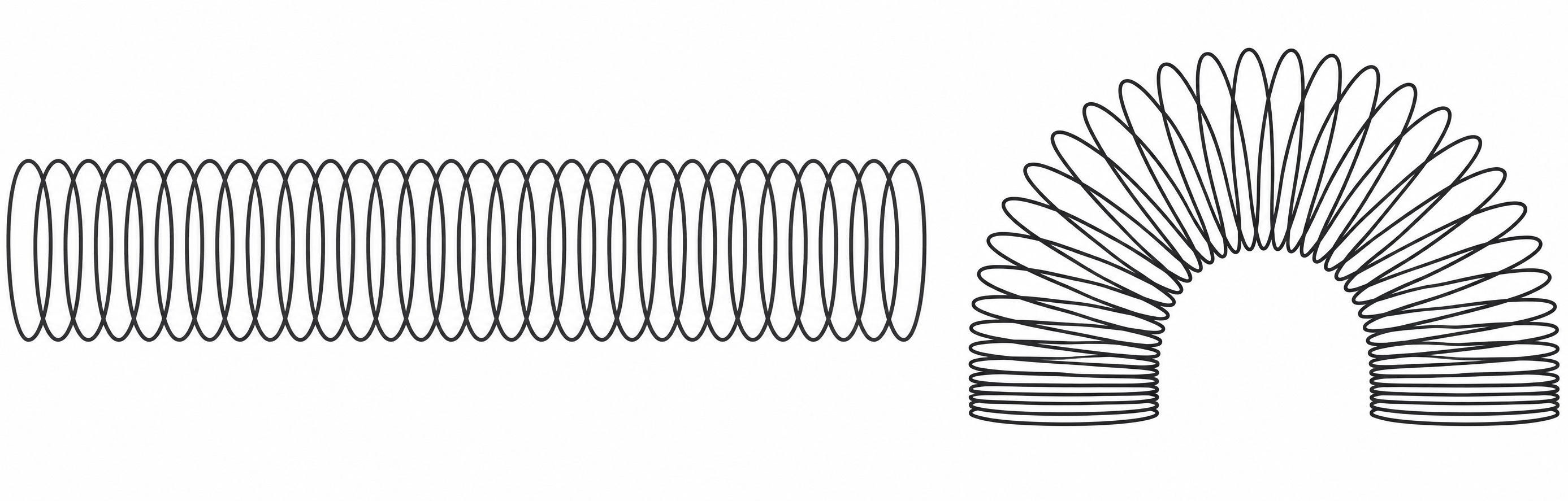
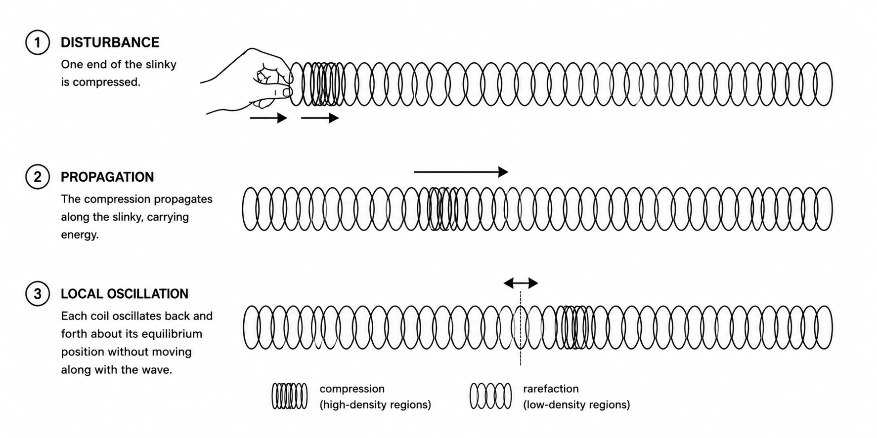
Among the various ones possible, one of the experiments that made me smile more than usual goes like this: you hold the Slinky at both ends and observe how a perturbation propagates from one end to the other.
If the game comes off well, it almost seems that the mass of compressed coils is always the same one, moving along the entire length of the spring. In reality no coil actually moves; each one merely oscillates around its own position, pushing the adjacent coil. Of course, we are talking about a longitudinal wave, but the aspect I find interesting to observe lies in the fact that each coil “transmits the information” only to the nearest ones. Even so, the effect crosses the entire spring.
And what if we tried to look at the neural network from the same point of view?
A neural network, when it is used, does something very similar. An input enters at one end, crosses the layers one after another, and produces an output at the other end. Each neuron receives the values from the previous one, combines them with its own weights, and passes the result to the next. The information always flows in the same direction, from input to output, like the compression along the Slinky.
We have already seen this in the chapter on neural networks; let us take up again a generic network with three hidden layers, a certain set of input data $\boldsymbol{x}$, the ground truth $\boldsymbol{y}$, and an activation function $a$.
When the information passes through the network, this is what happens:
$$ \begin{array}{c} \boxed{x} \\[4pt] \downarrow \\[4pt] f_0 = A_0 \cdot \underline{x} + \beta_0 \\[4pt] \downarrow \\[4pt] h_1 = a(\underline{f_0}) \\[4pt] \downarrow \\[4pt] f_1 = A_1 \cdot \underline{h_1} + \beta_1 \\[4pt] \downarrow \\[4pt] h_2 = a(\underline{f_1}) \\[4pt] \downarrow \\[4pt] f_2 = A_2 \cdot \underline{h_2} + \beta_2 \\[4pt] \downarrow \\[4pt] h_3 = a(\underline{f_2}) \\[4pt] \downarrow \\[4pt] f_3 = A_3 \cdot \underline{h_3} + \beta_3 \\[4pt] \downarrow \\[4pt] \boxed{\hat{y}} \end{array} $$where $A_l$ collects in matrix form the weights $\alpha^l_{kj}$, and the last step, $f_3$, stands in for the final combination with $\phi$ seen in the neural network articles.
We have also seen that if our network has to return a probability distribution, the last step would be:
$\hat{\boldsymbol{y}}=softmax(f3)$
But for simplicity, from here on we will refer to the network without this last step.
And what happens when a Slinky deforms in more than one place? It is not uncommon for our Slinky to end up with dents due to prolonged sessions of “experimentation” (try letting it dangle from a certain height and then release the end still in your hand, once the spring has reached its maximum extension).
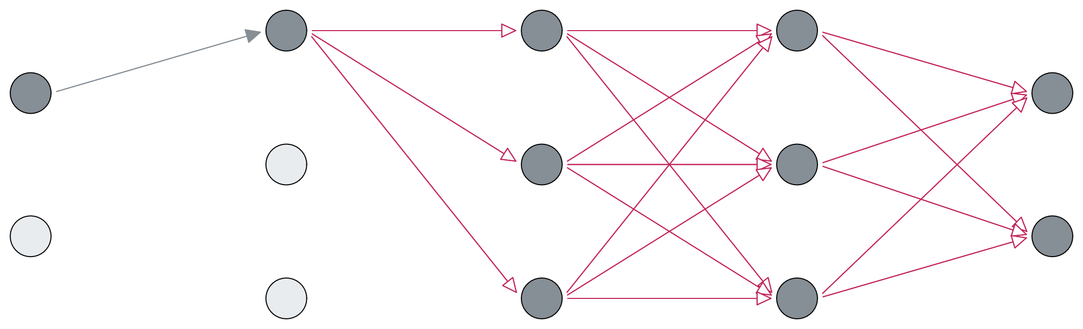
We said that each coil transmits the information about the movement to be made to the next coil. And it is clear that if one coil does not work, the push is modified, and so is that of the following coil, all the way down. Put differently: a local perturbation has turned into a change that runs through the entire spring, crossing all the coils that come after the damaged point.
And the interesting thing is that along the way, this “ripple” can grow or dampen, depending on how each stretch of the spring transmits it.
This is exactly the image that I would like to make clear the point I had only touched on in the previous articles.
Each weight multiplies the activation arriving from one unit and passes the result to the next unit. The effect of a small variation in that weight is therefore amplified or attenuated by the activation it encounters, and it propagates like a ripple through the whole network.
Looking back along the coils
Each weight therefore bears a share of responsibility for the final gap, and that responsibility is precisely the effect that its small variation produces at the end, after crossing the whole chain.
Measuring this responsibility means answering a question: if I changed this parameter by a tiny amount, by how much would the error change? It is the sensitivity of the error with respect to the parameter, which we write as the derivative of the loss $\mathcal{L}$ with respect to it.
$$ \frac{\partial \mathcal{L}}{\partial \theta} $$The larger this value, the more that parameter is responsible for the error, and the more it is worth acting on it. Correcting the network means shifting each parameter in proportion to this responsibility, in the direction that reduces the error.
Back to the Slinky, it is the work of someone who has to put the deformed coils back in place. There is no sense in looking at the coils one by one, hoping to guess by sight which one is off. It is better instead to start from what one observes beginning at the bottom, and from there work back up to understand how much each coil has actually contributed.
Here one also understands the meaning of the name backpropagation. The phenomenon, the ripple, goes forward, from the weight towards the output. But the calculation of responsibility is better done in the opposite direction. Here too it is better to start from the final gap and work back up to the first operation, because in this way the quantities already computed for the layers near the output are reused for the deeper ones, instead of redoing the whole path every time.
To understand how the error depends on a deep pre-activation, one works back up the chain, and each step reuses the work of the step nearest to the loss.
$$ \begin{aligned} \frac{\partial \mathcal{L}}{\partial f_2} &= \frac{\partial h_3}{\partial f_2}\, \underbrace{\frac{\partial f_3}{\partial h_3}\,\frac{\partial \mathcal{L}}{\partial f_3}}_{\text{from the loss}} \\[10pt] \frac{\partial \mathcal{L}}{\partial f_1} &= \frac{\partial h_2}{\partial f_1}\,\frac{\partial f_2}{\partial h_2}\, \underbrace{\left(\frac{\partial h_3}{\partial f_2}\,\frac{\partial f_3}{\partial h_3}\,\frac{\partial \mathcal{L}}{\partial f_3}\right)}_{\text{from } f_2} \\[10pt] \frac{\partial \mathcal{L}}{\partial f_0} &= \frac{\partial h_1}{\partial f_0}\,\frac{\partial f_1}{\partial h_1}\, \underbrace{\frac{\partial h_2}{\partial f_1}\,\frac{\partial f_2}{\partial h_2}}_{\text{from } f_1}\, \underbrace{\frac{\partial h_3}{\partial f_2}\,\frac{\partial f_3}{\partial h_3}\,\frac{\partial \mathcal{L}}{\partial f_3}}_{\text{from } f_2} \end{aligned} $$If we give a name to the quantity that accumulates, calling $\delta_k = \dfrac{\partial \mathcal{L}}{\partial f_k}$ the sensitivity of the loss with respect to the pre-activation of layer $k$, the reuse becomes explicit, because each $\delta$ is written starting from the previous one.
$$ \begin{aligned} \delta_2 &= \frac{\partial h_3}{\partial f_2}\,\frac{\partial f_3}{\partial h_3}\,\delta_3 \\[8pt] \delta_1 &= \frac{\partial h_2}{\partial f_1}\,\frac{\partial f_2}{\partial h_2}\,\delta_2 \\[8pt] \delta_0 &= \frac{\partial h_1}{\partial f_0}\,\frac{\partial f_1}{\partial h_1}\,\delta_1 \end{aligned} $$Here one sees at a glance that $\delta_2$ enters into $\delta_1$, which in turn enters into $\delta_0$, and that each step reuses in full the quantity already computed one layer nearer to the loss.
One also understands why the ripple we spoke of can dampen or grow along the way. Each step of the chain multiplies by a factor, and it is a product of many quantities lined up in a row. A product of this kind collapses towards zero when the factors stay on average below unity, and diverges when they exceed it. In the first case the correction does not reach the deeper layers, which stay almost still. In the second the training becomes unstable. It is exactly the stretch of spring that absorbs the wave until it dies out, or relaunches it until it swells. This phenomenon has a name, vanishing and exploding gradient.
The deeper the pre-activation, the longer the chain, but the path towards the loss is always the same and is computed only once. This is the meaning of “looking back”.
Seen this way, backpropagation is not just a technique for descending along a curve. It is the procedure by which a system seeks its own equilibrium configuration.
And let us be clear, a system that has reached an equilibrium is not, in itself, a system that produces correct results or works correctly. Let us not confuse the two things.
We will see this when we talk about Large Language Models and “hallucinations”. If for us it makes sense to speak of “correct” or “wrong”, it does not from the point of view of a model that brings out what its internal states propagate.
Historically, backpropagation arose long before reaching neural networks. Its genealogy passes through the optimal control theory of the 1950s and 1960s, Pontryagin’s adjoint method, and so on.
Only much later came the connectionist rediscovery by Rumelhart, Hinton and Williams in 1986 with the scientific paper “Learning representations by back-propagating errors”.
The mathematics of equilibrium (bonus paragraph)
When the repair is finished, the Slinky finds itself again in what we can regard, after various attempts, as a “stable configuration”. We can consider this configuration as the state in which the internal tensions balance out and the system reaches equilibrium.
In physics an equilibrium of this kind is described as the state that makes the system’s energy minimal. The condition is written by saying that the variation of the energy, for a small perturbation, is zero.
$$ \delta E(u) = 0 $$Where $u$ is the displacement or the deformation, and $E$ is the energy functional. It is the same language with which a great many equilibrium problems are described, from elasticity to membranes to stationary fluids, and from this condition one derives the equations that characterise the state of equilibrium, the so-called elliptic equations.
In mathematics there is an inequality, called the Caccioppoli inequality, that says something very intuitive about a system in equilibrium and that ties in precisely with the ripple we have talked about. In a Slinky at rest, the internal deformation cannot grow at will without the overall state of the system revealing it. How deformed things are locally is kept under control by how deformed the configuration is as a whole. A system in equilibrium, in other words, cannot hide internal tensions.
the Caccioppoli inequality, in brief. For the solutions of the equilibrium equations (the elliptic PDEs), the inequality controls the energy of the deformation over an inner region starting from the values of the function over a slightly larger region. In simplified form, on a ball of radius $R$, it is written $\int |\nabla u|^2 \leq \frac{C}{R^2} \int |u|^2$, with the integral on the left over the inner region and the one on the right over a larger one. It is also known as the reverse Poincaré inequality, because it goes in the opposite direction to the usual one. Normally one controls a function starting from its derivatives; here instead one controls the derivatives, that is the deformation, starting from the function alone, that is the state. This inequality characterises the state of equilibrium, that is the destination towards which the system settles, not the procedure by which one gets there. It speaks of what the equilibrium is like, not of how it is reached.
Naturally the Caccioppoli inequality lives in the field of elliptic equations and describes equilibrium solutions, that is the final state of a system, not the procedure by which a network is trained.
As a side note, I should point out that there is a line of research that uses neural networks to solve precisely these variational inequalities, that is the constrained equilibrium problems that generalise the condition $\delta E(u) = 0 $ seen above. It is a point at which the two halves of this article, the networks and the mathematics of equilibrium, end up touching. With the usual caveat: there the network is merely the tool that approximates the equilibrium solution, while the equilibrium remains the destination, not the procedure.
For those who want to get an idea, an example is: Zhao e Zheng,Neural Network Convergence for Variational Inequalities (preprint, 2025).
I wanted to write this addition because the concept of equilibrium reminded me of the figure of Renato Caccioppoli. Besides having been one of the most important Italian mathematicians of the twentieth century, he was one of those intellectual figures who taught me to trace an ever-wider neighbourhood around my thoughts.
Maybe it’s a superfluous addition, maybe it’s a cue, maybe it’s just strange and then that’s enough.