(On folding paper creatively and, along the way, understanding neural networks)
We know more or less from history that one day some guy discovered that by melting minerals you could stop chipping flint, and that over time everyone came to understand what metals were, even without being a blacksmith.
Another day some guy discovered that wheels roll, another that presses press, and yet another that industries industrialised. And we could say, without a shadow of a doubt, that over time, grasping the intuitive part of every technological leap has remained something potentially within anyone’s reach.
Computers, too, for all their digital nature, maintain an “analogical” approach: if some guy clicks a button on a web page, he has more or less a clear intuition that somewhere another guy once figured out how to program it, on a computer that yet another guy invented, to transmit his gesture to the machine as a series of finite states.
With Artificial Intelligence, no: that understanding between new technologies and human beings has broken down. In most cases, a response from a chatbot based on a Large Language Model is considered magic. We know that more or less somewhere, other guys are performing esoteric rituals that are hard to get even a vague intuition about.
This is the first in a series of articles/experiments on artificial intelligence that aim (or at least attempt) to restore that layer of intuition that should connect people to the technology they use. Starting from the personal assumption that, to have a correct understanding of AI, it is necessary to understand what we are actually talking about from a mathematical point of view.
If there is one thing I have always admired about mathematicians like Israel Herstein (known for making abstract algebra accessible without betraying its rigour), it is the clear intention in his texts to make a subject understandable that many find hopelessly intimidating. Since for me mathematics is a strange and wonderful form of painting, let’s see whether, without sacrificing too many formulas, we can give a description of a technology that has by now reached everyone. Naturally, the style will be closer to “Herstein explains algebra in a roman trattoria”.
So, with the preamble out of the way, the topic of this first article is: neural networks.
We will see that they are nothing more than origami made of equations, and that understanding this does not require being a mathematician, just the patience to fold a sheet of paper.
What makes this teddy bear truly cuddly?
On one side, a teddy bear; on the other, a curve obtained by plotting a set of input data $\boldsymbol{x}$ against a set of data $\boldsymbol{y}$.
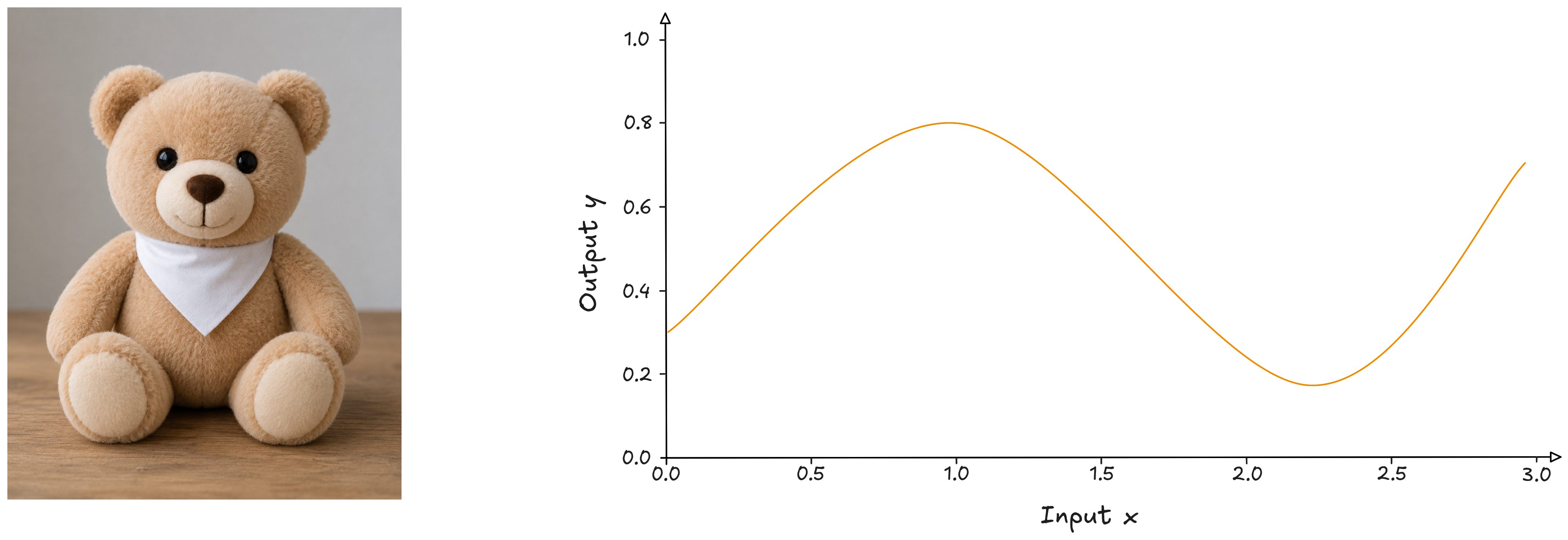
Is there a way to capture the cuddly essence of a teddy bear with an origami? If I managed it, I would have a model capable of reproducing a base from which to build an army of teddy bears, with the possibility of adding new consistently cuddly characteristics along the way.
That curve, on the other hand, could be the product of a mathematical function that generates it. How do I grasp the essence of that curve? We will call this function $y = f(x)$. We do not know it, but if we managed to model it, we would have a function capable not only of replicating the known data, but also of generating new data consistently with the context in which the original data lives.
A blank sheet and a straight line
We are making an origami, and where better to start than with a blank sheet of paper. First step: let’s fold it in half.
We proceed the same way on the mathematical side: we want to reach an ideal function, but without wandering through theorems, let’s start from a very, very simple equation: the straight line.
$$ y = \alpha \cdot x + \beta $$where:
- $x$: the part of the dataset representing the inputs
- $y$: the outputs I know and will use as examples
- $\alpha$: the slope coefficient, the value whose change shifts the line’s orientation
- $\beta$: the intercept, the value that moves the line away from the origin, pushing it up or down depending on its sign
When we study this kind of equation at school, we look for a value of $x$ such that, once substituted into an expression whose $y$ we already know, it makes that expression true. For example: in $2x + 3 = 7$, the value that satisfies the expression is $x = 2$.
But here things are different: we know both the input data and the output data. This is where everything changes: we are no longer looking for the unknown in the input, but in the model’s parameters. The values to find are $\alpha$ and $\beta$.
We will call these values parameters, and finding them will determine the success or failure of our model.
So in the end, regardless of complexity, I will have a model that, starting from the input data $\boldsymbol{x}$ and having found the right parameters $[\alpha, \beta]$, produces results consistent with the output $\boldsymbol{y}$.
$$ \begin{align*} y &= f(x, \alpha, \beta) \\ &= x \cdot \alpha + \beta \end{align*} $$Well begun is half done…
Now, if I think about a parameter to factor into my origami, the first one is certainly the rotation of the sheet. Going by intuition and working with angles, I could have many more possibilities for representation.
Of course, we are still far from the image of a teddy bear, but if I look at the original and rotate the sheet 45 degrees, it already gives the impression of containing the final result.
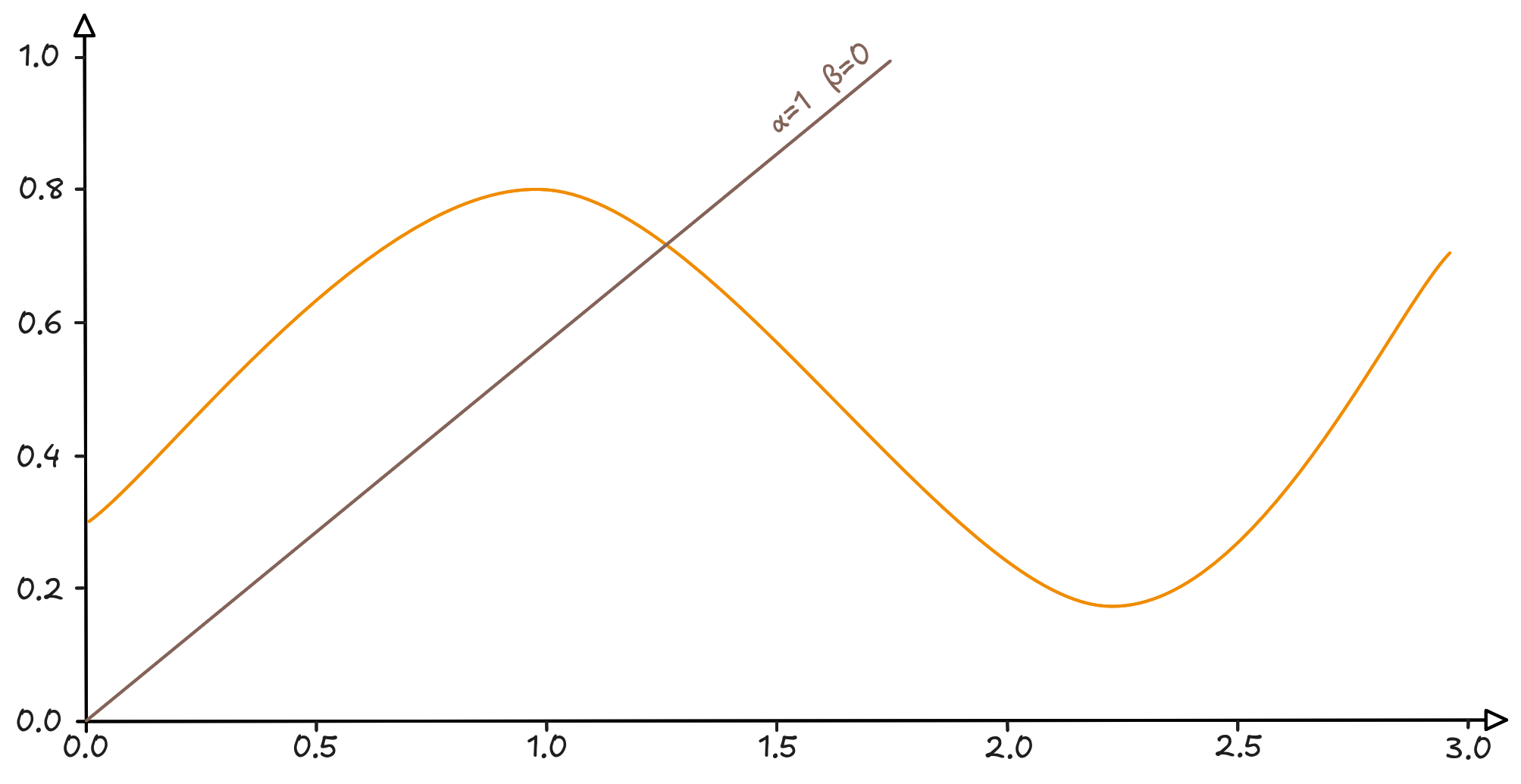
Meanwhile, if I think about the two parameters of the line, we notice that changing their value is a bit like sliding it up and down the graph, rotating until I find the position that best “captures” the curve.
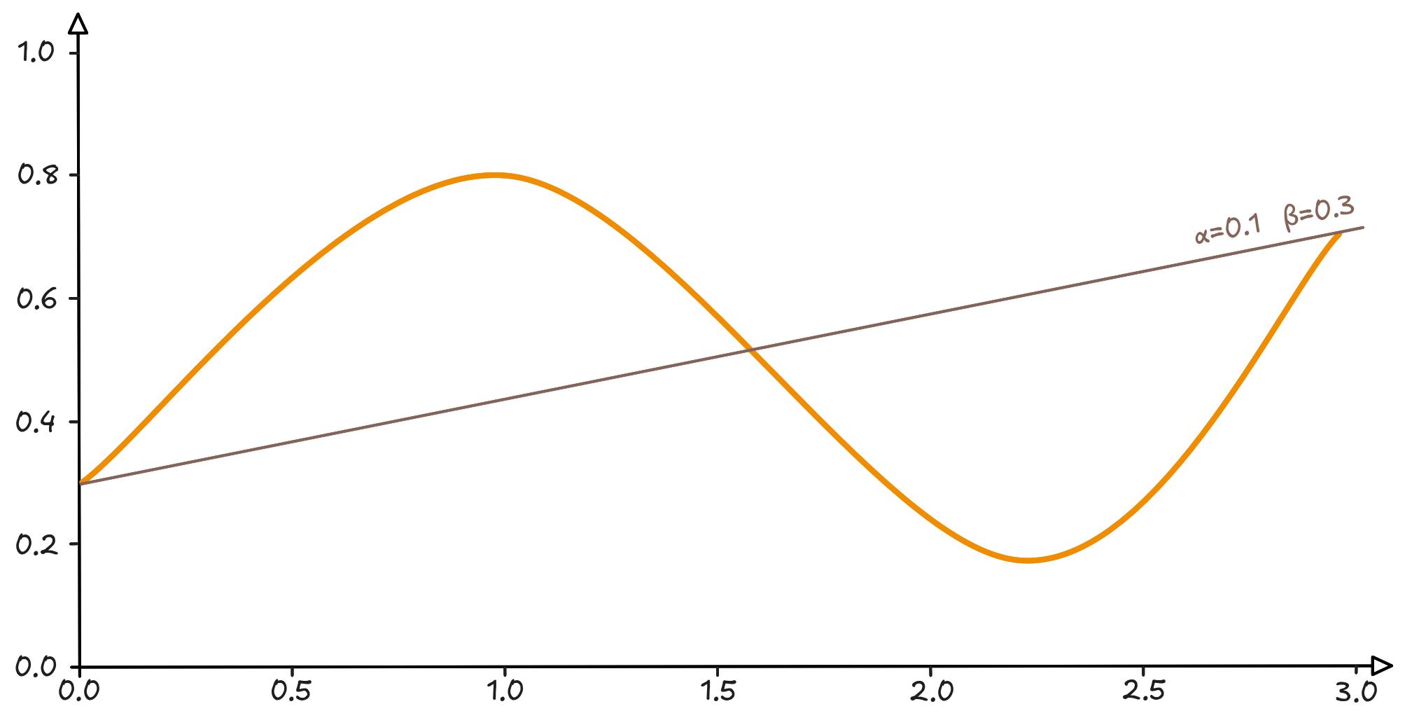
Not bad. We found a line that passes exactly through the middle of the curve.
Can we consider it a summary? Absolutely yes. Let’s try to grasp a fundamental point: the line passes more or less through the middle and divides the curve into two more or less equal halves. In other words: the error I make by approximating the curve with the line $y = 0.1x + 0.3$ is quantifiable, and we could eventually find a way to describe it.
So, can we be sure that by extending the line, the approximation error for new points will be consistent with that on the known ones? The most fitting answer to this question is, and always will be: Definitely Maybe.
Let’s make one thing clear, a concept I personally believe should be carved in stone every time we talk about AI:
“the only two words that matter in Artificial Intelligence are: acceptable and negligible”.
It must be understood, and we will come to understand it along the way, that no matter how refined or complex a model may be, it will always carry a margin of error that, however minimised, can never justify anyone uttering the fateful words: “our solution reaches an accuracy close to 100%”. If you ever hear that sentence… run!
Folding along the edges
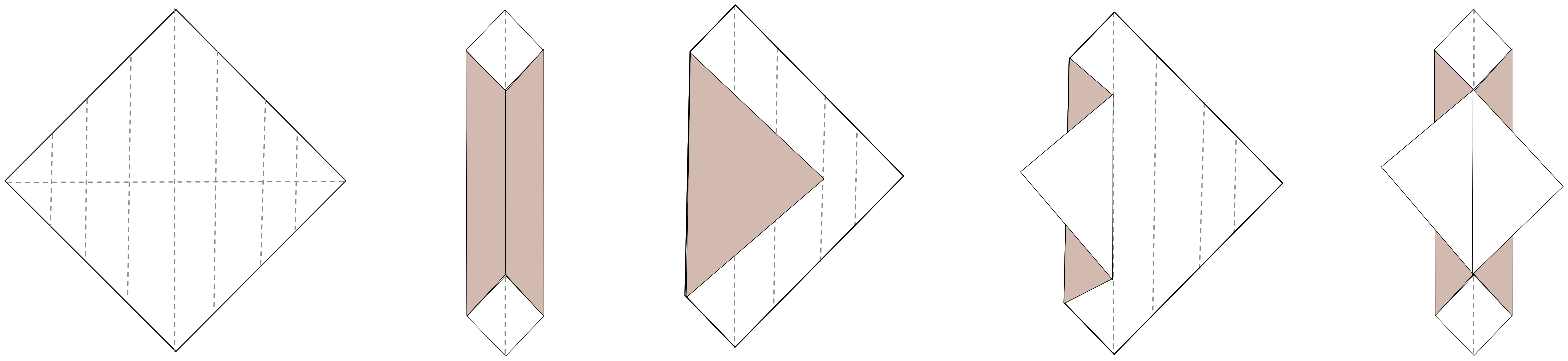
It is time to give structure to our origami. We need to choose the initial folds, those that will guide all the subsequent steps. Let’s start by creating four distinct, well-positioned zones capable of containing the detail folds.
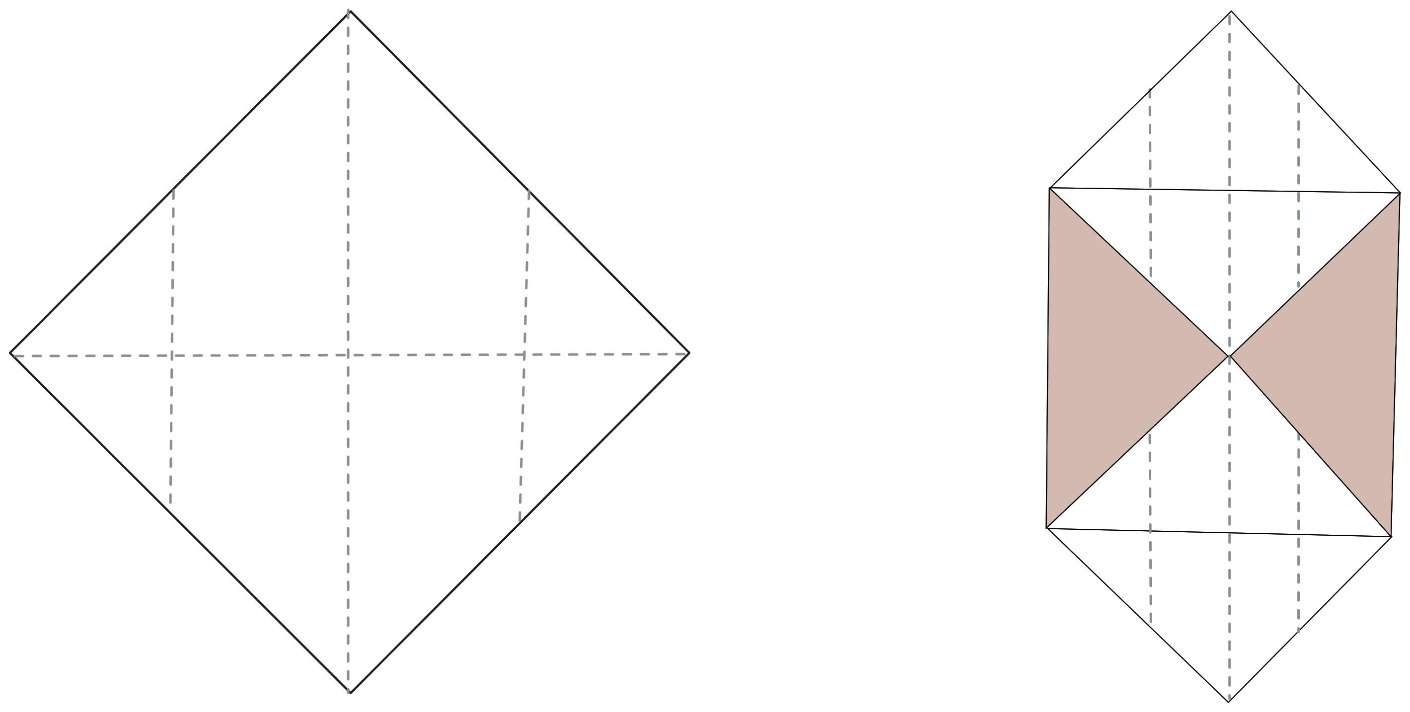
Notice that the active folds, the outermost ones, open up the possibility of evolving our structure and creating new geometry to work with. The two inner folds are, for now, inactive, but they are there, and in subsequent steps they will certainly come in handy.
And for the curve? I proceed with exactly the same logic. It is clear that a single line is not ideal for representing a curve, so why not “fold” it to carve out four well-defined zones?
Let’s start by going from one line to three equations:
$$ \begin{align*} h_1 &= x \alpha_1 + \beta_1 \\ h_2 &= x \alpha_2 + \beta_2 \\ h_3 &= x \alpha_3 + \beta_3 \end{align*} $$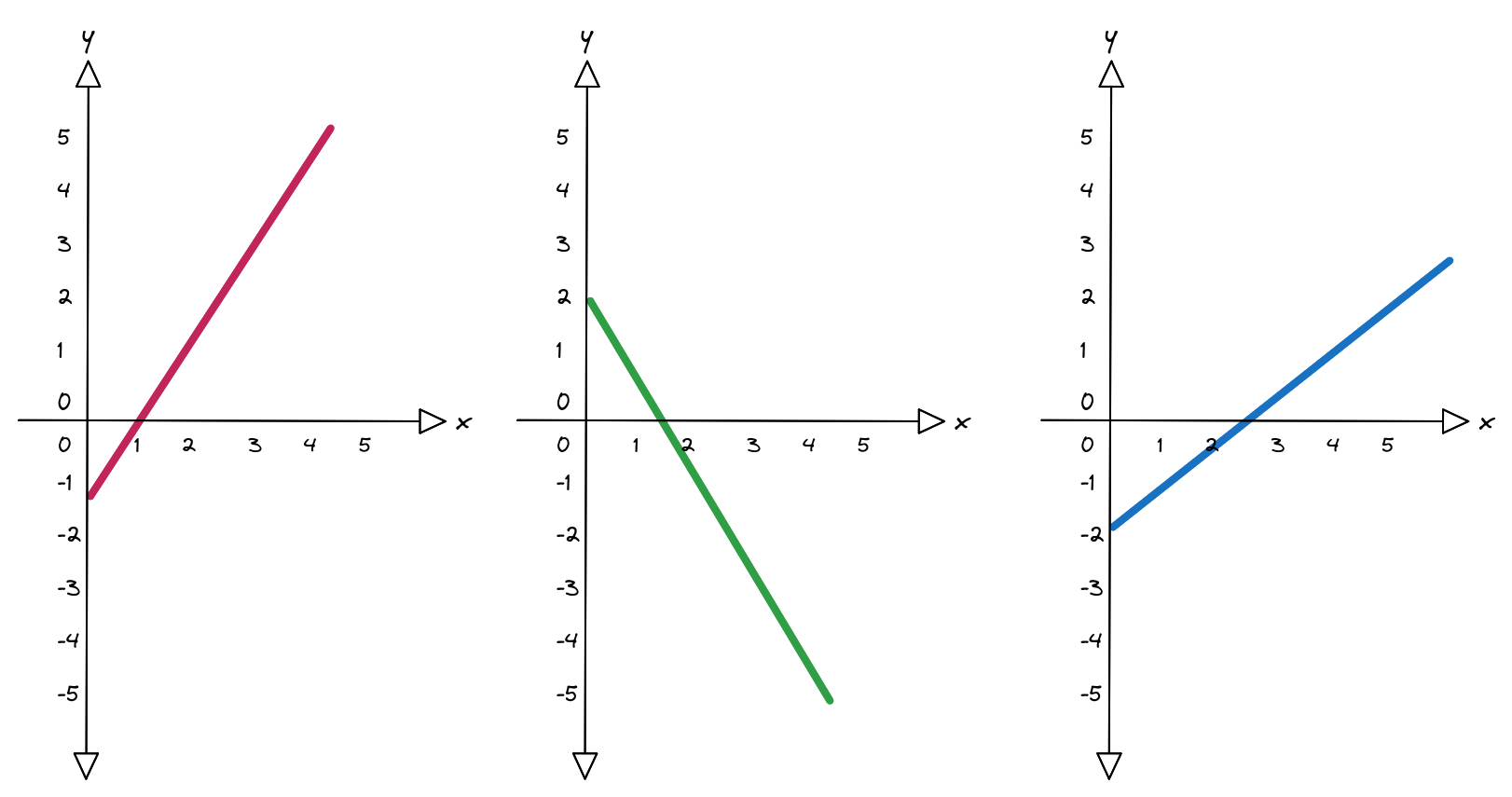
We now have three equations, but we need to account for the fact that, being three continuous lines, it is somewhat complicated to understand how to join them. We would need to insert some breakpoints, junction points at which to connect the three equations.
First, let’s draw a distinction, a simplified one, but necessary for understanding what follows. A linear relationship between input $x$ and output $y$ changes in a constant, proportional way: double the cause, double the effect, forming a straight line on the graph. A non-linear relationship, on the other hand, changes variably, forming curves or oscillations. In this case, small initial changes can lead to enormous or disproportionate final results.
There is a problem, though: adding linear functions always produces a linear function. If we combined the three lines as they were, we would end up with a single line, more complicated to compute but just as rigid. To truly “fold” the equations, we need something that introduces a discontinuity, a point where behaviour changes.
Let’s try to draw something useful from all this.
- Moving from a linear to a non-linear representation is useful for composing lines in a way that brings us closer to the target curve.
- Non-linearity brings great power but also great responsibility (small changes can lead to unusable results).
- We have seen in our origami that some folds are active and some are not. It would therefore be useful to assign a weight to each equation so as to “shape” its contribution at any given point.
In short, we are looking for a function that transforms our functions from linear to non-linear.
The answer is called an activation function $a(x)$: a family of tools capable of introducing exactly the discontinuity we need. In our case, we will use the Rectified Linear Unit ($ReLU$).
$$ a(x) = ReLU(x) = \begin{cases} 0 & x < 0 \\ x & x \ge 0 \end{cases} $$If $x$ is greater than zero, then $y = x$; otherwise, if $x$ is less than zero, then $y = 0$.
We can now rewrite:
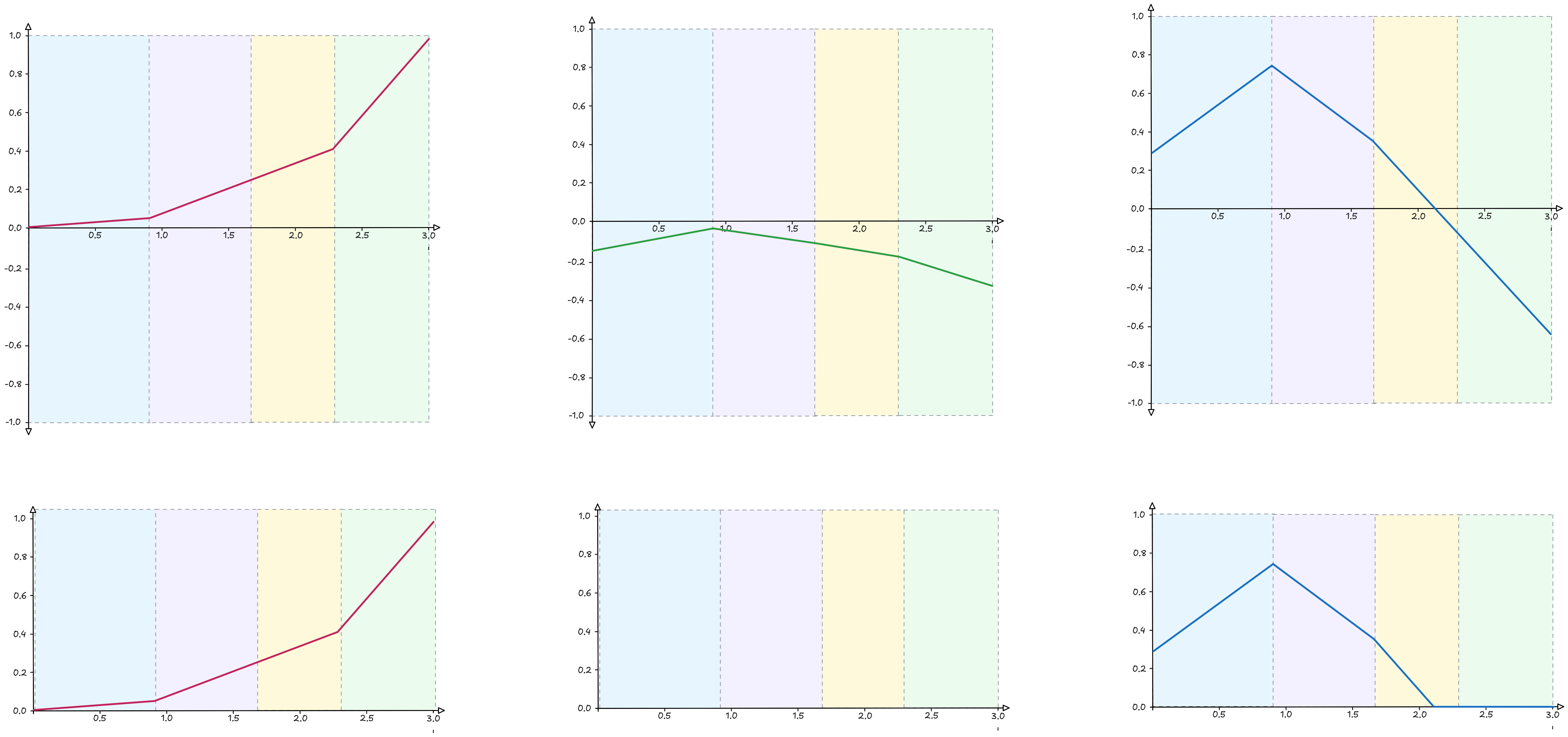
$$ \begin{align*} h_1 &= a(x \alpha_1 + \beta_1) \\ h_2 &= a(x \alpha_2 + \beta_2) \\ h_3 &= a(x \alpha_3 + \beta_3) \end{align*} $$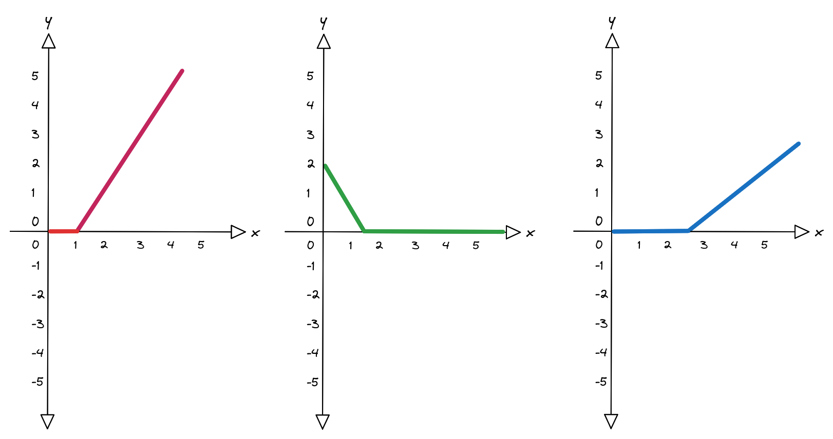
We now need to combine the three equations, but first we need to understand how to weight the actual contribution of each one. The simplest way is to add new parameters to find, in order to quantify this contribution. We will call $\phi_n$ this set of parameters and use them within the following combination:
$$ \begin{align*} y &= \phi_0 + \phi_1 h_1 + \phi_2 h_2 + \phi_3 h_3 \\ &= \phi_0 + \phi_1 a(x \alpha_1 + \beta_1) + \phi_2 a(x \alpha_2 + \beta_2) + \phi_3 a(x \alpha_3 + \beta_3) \end{align*} $$Let’s make sure we understand what has happened so far:
- we started with a straight line
- we transformed it into three folded pieces where:
- the parameters $\alpha$ and $\beta$ define the base functions
- the parameters $\phi_n$ decide how much each function contributes to the final result
- we then combined these three pieces linearly
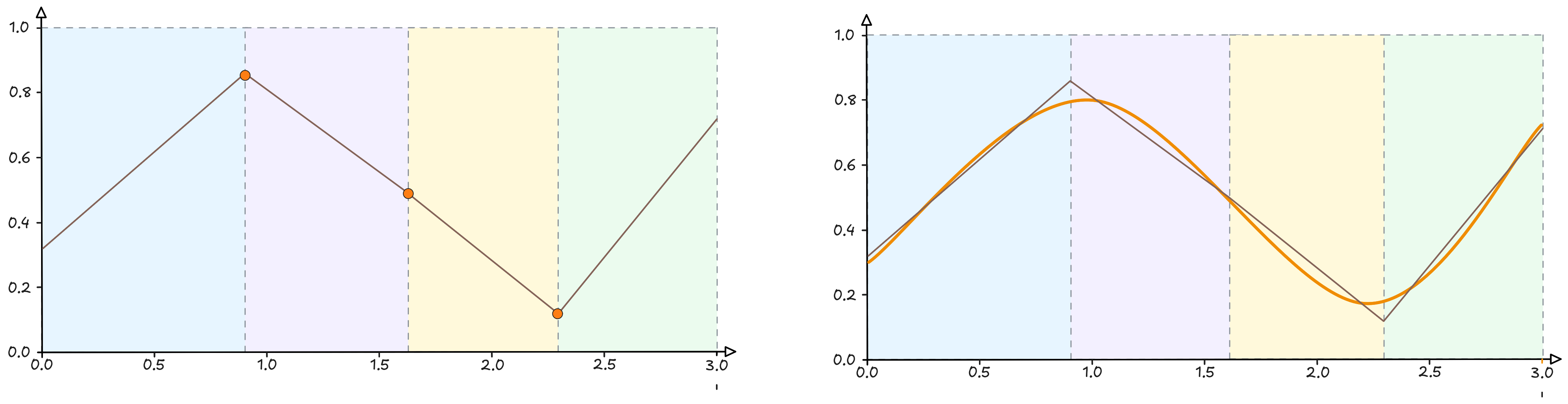
The result is a final function made up of at most four linear segments in (x).
Much like in origami, we have created four zones within which to start defining the folds needed to reach our goal.
The difference worth noting is that in the origami case we have two active folds and two inactive ones; in our mathematical origami, however, all folds are active and contribute to the final shape.
I would like to close this section by adding one final layer of complexity. The formula below generalises everything written so far:
$$ y = \phi_0 + \phi_1 h_1 + \ldots + \phi_n h_n = \phi_0 + \sum_{i=1}^{n} \phi_i h_i $$The symbol $\sum$ (sigma) is nothing more than a compact way of describing a sum of elements from 1 to $n$.
Infinity is not a thing, but a possibility that never runs out
The actual quote by mathematician Henri Poincaré is this:
In reality infinity does not exist, and when we speak of an infinite collection, we mean a collection to which we can continually add new elements. (The Logic of Infinity, 1912)
Poincaré conceived of infinity not as a completed object but as a process: something to which one keeps adding, without ever exhausting it. I like using this idea (even though it was largely set aside by twentieth-century mathematics, in favour of Cantor’s conception of infinity) to describe how a neural network decomposes complex information through successive layers, each of which does not exhaust the meaning but passes it on to the next, enriched. If nothing else, it’s a very… human association of ideas.
But let’s return to our origami. We have reached a point where the previous steps will determine the ones that follow. The rough folds certainly do not define a figure, but, as already mentioned, each of those generated areas will be the foundation for building increasingly refined details.
The same applies to our model: we need to refine the previous result to bring it even closer to the target curve.
We start by building a new series of functions capable of generating further “folds” within the previous ones, that is, a second layer of functions whose input will be the output of the previous layer.
Before proceeding, let’s adopt a convention to distinguish parameters between layers: we will use the first-level parameter $p'$ for the first layer and the second-level parameter $p''$ for the second.
We rewrite the first layer as follows:
$$ \begin{align*} h_1' &= a(x \cdot \alpha_1' + \beta_1') \\ h_2' &= a(x \cdot \alpha_2' + \beta_2') \\ h_3' &= a(x \cdot \alpha_3' + \beta_3') \end{align*} $$We now move to the second layer. Here too, the result comes from a linear function transformed by an activation function $a(x) = ReLU(x)$.
$$ \begin{align*} h_1'' &= a(y' \cdot \alpha_1'' + \beta_1'') \\ h_2'' &= a(y' \cdot \alpha_2'' + \beta_2'') \\ h_3'' &= a(y' \cdot \alpha_3'' + \beta_3'') \end{align*} $$But we already know how to compute $y'$: it is the linear combination of the first-layer functions, that is, $y' = \phi_0' + \phi_1' h_1' + \phi_2' h_2' + \phi_3' h_3'$.
Substituting this expression into each $h_n''$, we get:
$$ \begin{align*} h_1'' &= a(\phi'_{10} + \phi'_{11} h_1' + \phi'_{12} h_2' + \phi'_{13} h_3') \\ h_2'' &= a(\phi'_{20} + \phi'_{21} h_1' + \phi'_{22} h_2' + \phi'_{23} h_3') \\ h_3'' &= a(\phi'_{30} + \phi'_{31} h_1' + \phi'_{32} h_2' + \phi'_{33} h_3') \end{align*} $$Note a subtle step here: in the original definition each $h_n''$ depended only on the scalar $y'$. Once $y'$ is expanded, however, each unit of the second layer depends separately on all three $h'$ of the first. By treating the $\phi'_{nj}$ as free, independent parameters we make exactly this leap: we move from a single “bottleneck” to a fully connected layer.
Our new output $y''$ will therefore take the following form:
$$ y'' = \phi''_0 + h_1'' \phi_1'' + h_2'' \phi_2'' + h_3'' \phi_3'' $$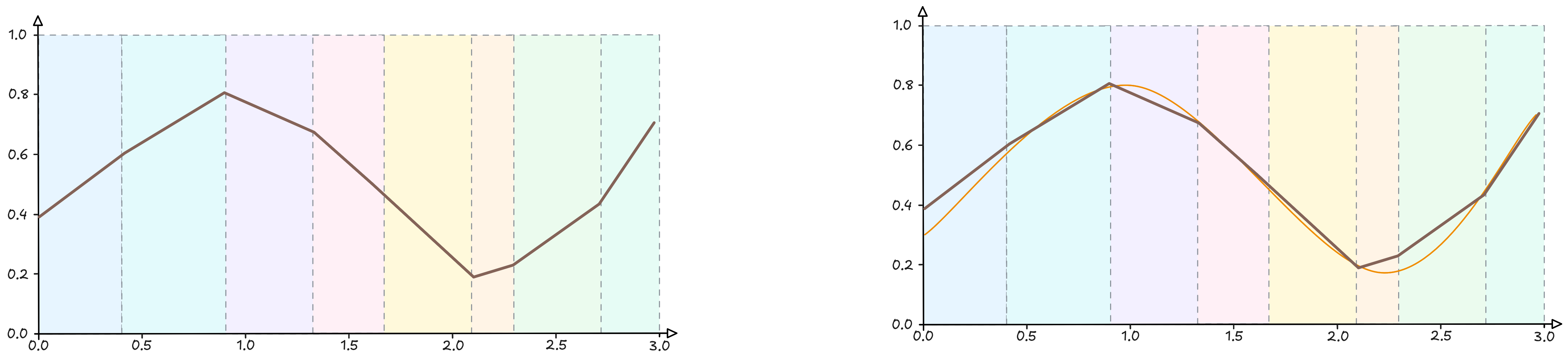
Two important observations arise from this last step:
-
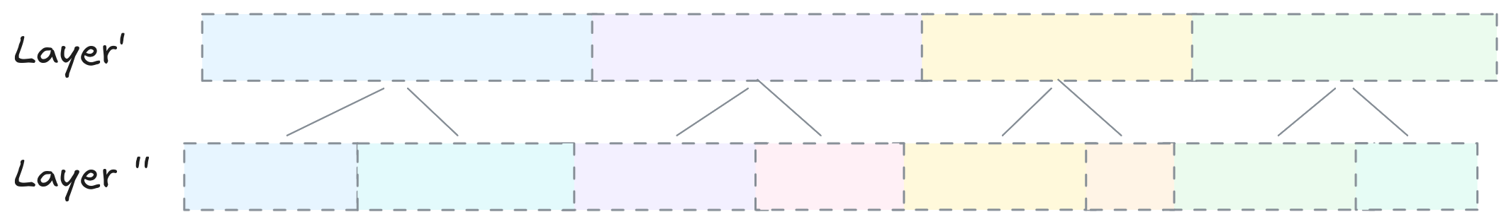
The new functions operate within the four zones defined by the previous layer, creating new ones within them. In the end we will obtain an approximation of the curve that is increasingly close to the original, by composing many small, well-defined pieces.
-
In the second layer it happens that the function $h_2''$ is not active (if the reason is not clear, go back to the description of the $ReLU$ function). This means that the first layer detected a feature, but the next layer determined that this feature, alone or in combination with the others, was not sufficient to activate.
At this point we could continue indefinitely (this time in Cantor’s sense), arriving at an ever more refined approximation of the curve, but this is not important for our purposes.
What I would like to make clear, however, is what we have achieved from a mathematical point of view: an enormous composition of simple mathematical functions.
So, about these neural networks…
Now let’s bring together every element of this composition of functions in a graphical representation that makes things easier to visualise.
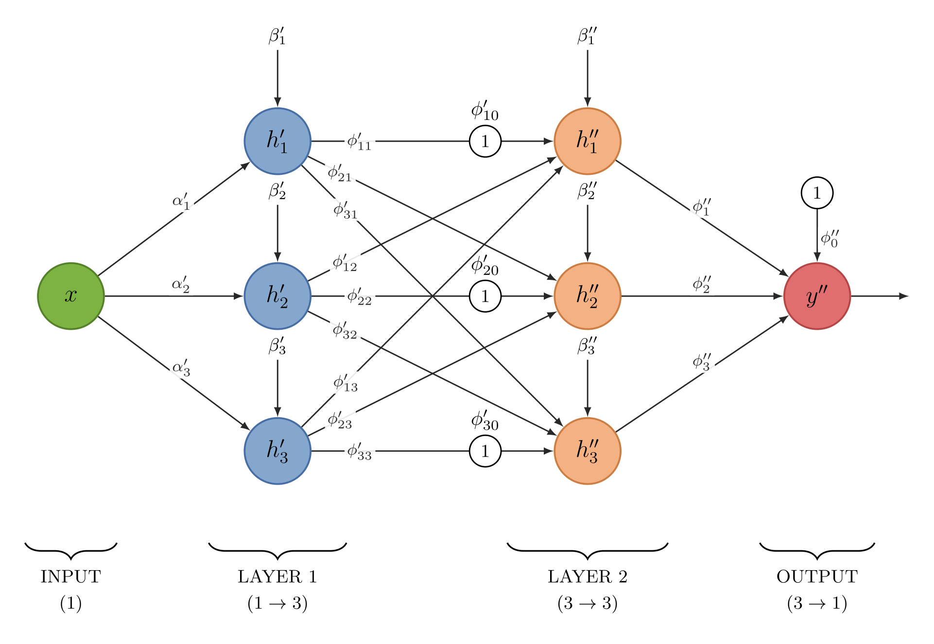
And there, at last, is the neural network.
No, you will not find illustrations of synapses here. I am by now convinced that it is a misleading representation. From my point of view, a neural network relates to the human brain the way a pigeon relates to an aeroplane. Birds certainly inspired the construction of aircraft, but walking under a flock of planes is not quite as risky as walking under a flock of pigeons that have just had lunch.
After all, the definition of a neural network is formalised in a theorem, the result of contributions starting with George Cybenko in 1989 through to Allan Pinkus in 1999.
Universal Approximation Theorem
For any continuous function on a compact subset of $\mathbb{R}^n$ and for any arbitrarily specified precision $\varepsilon > 0$, there exists a network with a single hidden layer containing a finite number of hidden units with a non-polynomial activation function, capable of uniformly approximating the given function to within that precision.
We can rewrite it more simply: however complicated a continuous function may be, there always exists a neural network with a single hidden layer capable of approximating it to whatever precision we desire, provided we use enough neurons and a suitable activation function.
In other words: neural networks are universal approximators. Whatever form the function we wish to model may take, the network can always get as close to it as we want, simply by increasing the number of hidden units.
I am convinced that the ability to give an intuitive representation of neural networks broke down precisely at this point, and that the problem lies in the choice of vocabulary. Calling the computational units “neurons” and the optimisation process “learning” certainly made the inspiration clear and helped spread the technology, but made it harder to genuinely understand what is actually happening. An artificial neuron does not think, does not perceive, does not remember: it performs an operation on a number and passes the result to the next layer. Machine learning does not learn the way a child learns: it adjusts parameters until the error falls below an acceptable threshold. The mathematics was accessible, the vocabulary made it opaque.
To be clear, this does not make neural networks any less complex, but we need to understand where the complexity actually lies. We are looking for mathematical models capable of capturing both the topology of a simple curve and that of extraordinarily complex constructions whose results we can observe but whose inner workings we struggle to imagine. I know that put this way it sounds like a contradiction. In reality, it is a bit like astrophysics: reducing years of research to the phrase “there is life on that planet” strips away the depth of everything that has been studied and of how much there is still left to understand.
But it doesn’t end there
When learning an origami, we start creating smaller and smaller folds, trying to reach a geometric configuration capable of capturing the essence of the original figure. The final result is therefore not a perfectly identical reproduction, but rather a coherent set of details that make us say: “this is a cuddly teddy bear”, or “this is a hungry grizzly that is decidedly not cuddly”.
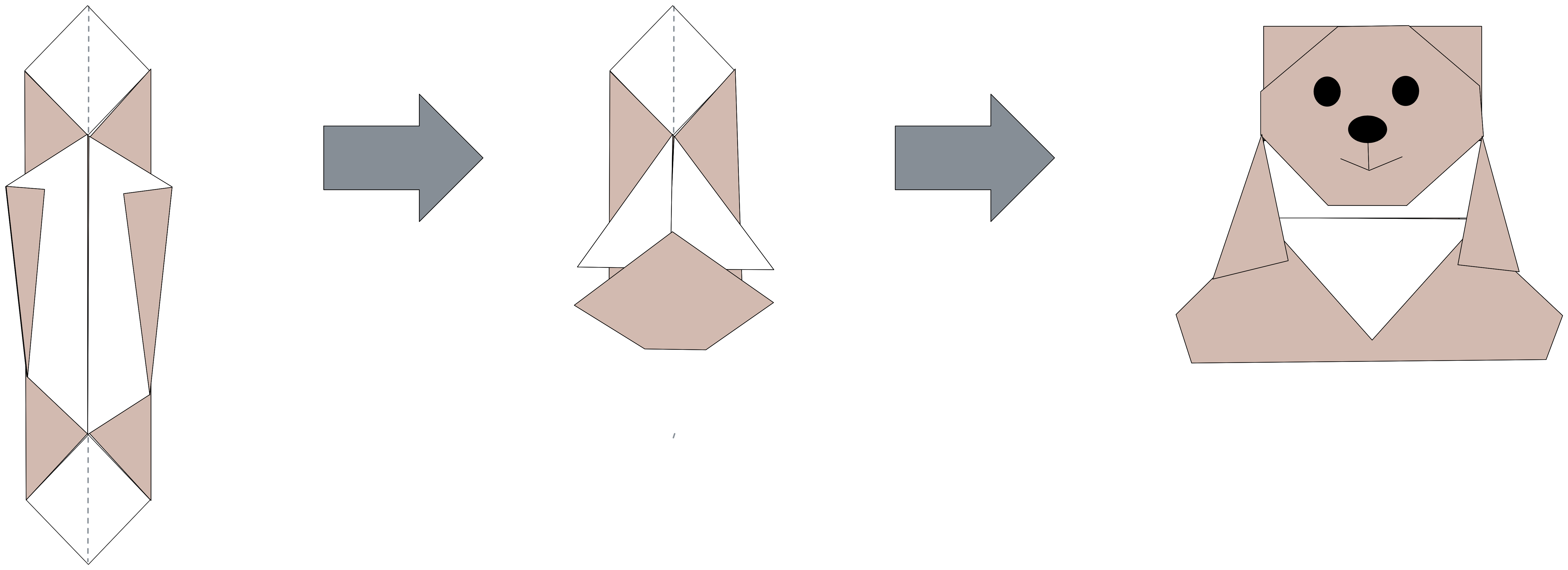
Forgive me, I have skipped through the steps. Anyone wishing to explore the origami pattern in full can find it here: https://www.supercoloring.com/it/media/paper-craft/456115/istruzioni-per-creare-un-origami-a-orsacchiotto
The same applies to our model. Each layer of functions $h_n$ specialises on a precise zone of the data space: each unit activates only when the input falls within that zone, remaining inactive otherwise. In this sense we might say that each unit “recognises” a specific configuration; everything else is ignored. It is this structural selectivity, multiplied across thousands of units and dozens of layers, that gives the network its capacity to approximate complex functions. All of this, until we reach a result that seems acceptable in terms of accuracy, with a negligible margin of error.
And how do we give shape to these two concepts? That is what we will see in the second part.
But I can offer you a preview. I am not good at origami, and my first attempt is almost always a disaster.

I am so bad at it that I had to ask an AI to generate an image of a badly made origami. But it is certainly a matter of parameters and how to find them.
Key terms
- Layer: a level of the neural network composed of a set of hidden units operating in parallel on the same input. Layers are chained: the output of one becomes the input of the next.
- Hidden unit: a neuron belonging to an intermediate layer of the neural network, not directly visible in either input or output.
- Linear function: a function of the form $f(x) = ax + b$, which produces a straight line in the plane.
- Activation function: a non-linear function applied to the output of each hidden unit to introduce non-linearity into the model.
- ReLU (Rectified Linear Unit): an activation function defined as $f(x) = \max(0, x)$. It returns the value unchanged if positive, otherwise zeroes it out, “clipping” the function below zero.
- Clipping: the process by which ReLU zeroes out the negative portion of a linear function, making it flat below zero.
- Kink: the point where the function changes slope, that is, where the line crosses zero and is clipped by the ReLU.
- Linear region: an interval of the input over which the output function behaves linearly, that is, between two consecutive kinks.
- Activation pattern: the combination of active and inactive units over a given interval of the input.
- Active/inactive unit: a hidden unit is called active when its value is not clipped by the ReLU (positive zone), and inactive when it is zeroed out (negative zone).
- Parameters φₙ: the weights by which each clipped line contributes to the final output function.
- Offset parameter φ₀: an additive constant that shifts the entire output function vertically.