It's all about the Entropy of Coffee

(How to have breakfast in southern Italy and understand the way neural networks classify)

foreword: this article continues the discussion started with neural networks: part 1 part 2. It might also turn out a little more demanding, so if something doesn’t add up, write to me.

I was born in a southern Italian region (Puglia), where coffee is a religion. But not simply “coffee”. Coffee made a certain way, and above all hot. Actually, not even hot. Scalding.

Coffee has to be scalding, and ever since I was little I witnessed my grandfather’s exhausting struggle with time. In winter especially, my grandfather had to fight against time. Time passed and the coffee cooled down, there was no solution. One moment too many spent watching television and the coffee was ruined.

Years later I would have liked to console my grandfather by explaining that there is no fundamental force explicitly forbidding coffee from spontaneously heating itself up off the table. The microscopic laws of physics allow it in principle. However, for a macroscopic system like a cup of hot coffee, it would require an extraordinarily improbable statistical fluctuation of entropy. Put more simply: the probability is so small that the phenomenon is enormously improbable.

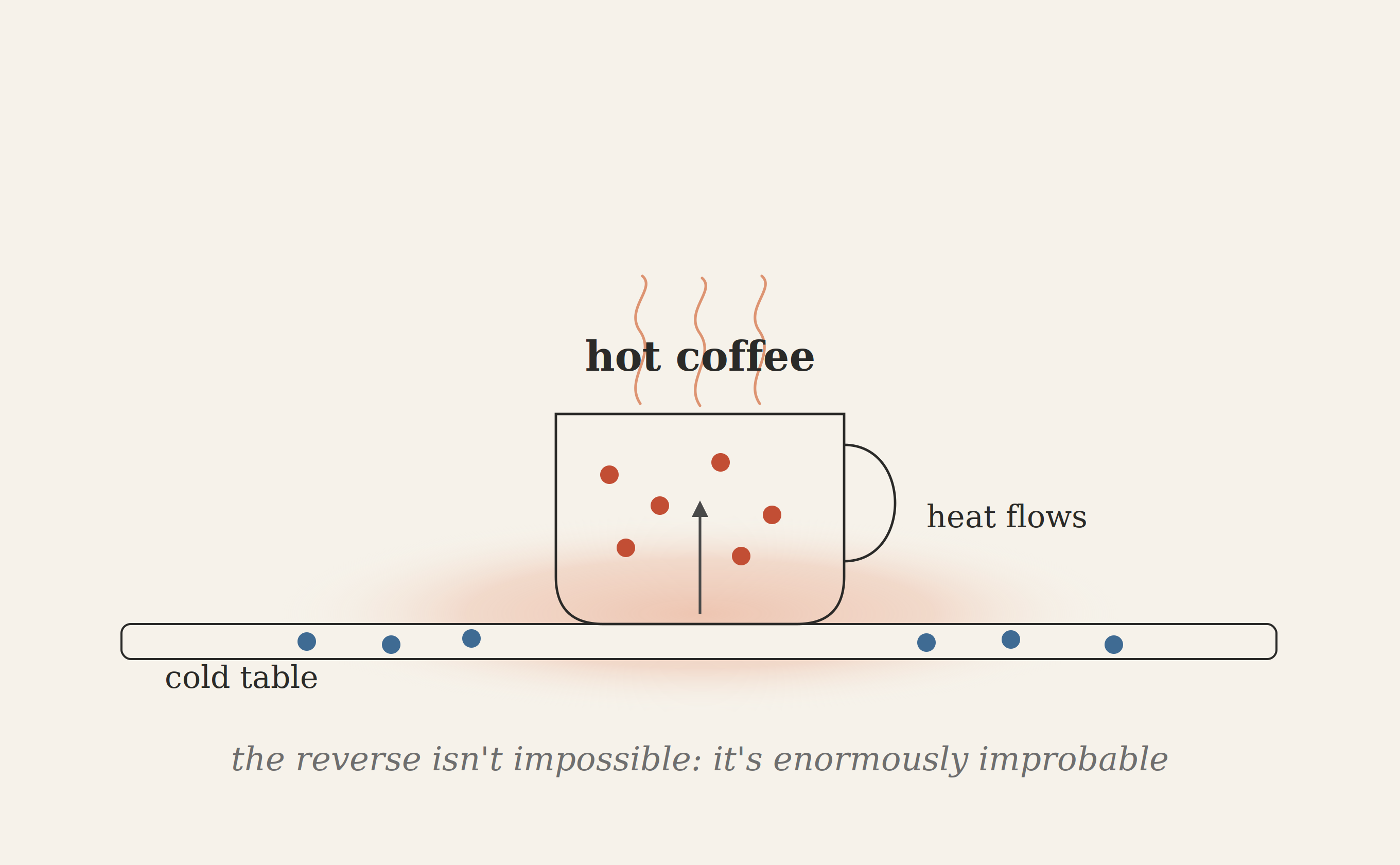
The laws of physics at the microscopic level are reversible: if I filmed the collisions of every single molecule and played the film backwards, every single collision would still be perfectly valid according to Newton’s laws. It is only at the macroscopic level, where what matters is the aggregate probabilities over billions upon billions of molecules, that one direction becomes predominant and therefore more probable than the other. It is not a law in the sense of a prohibition. It is a fluctuation the system simply never performs, for reasons of probability, not of principle.

The idea that the certainty we observe is the product of an enormous quantity of probabilistic events brings us back to where we left off in the articles on neural networks.

When a neural network has to choose a category, it doesn’t return a certain answer, but a distribution over all the possible answers. And it isn’t so different from my grandfather’s cup of coffee. The coffee too “returns” a direction for the flow of heat without any law explicitly imposing it.

There are many didactic representations for introducing the ways a neural network “classifies”, and for the most part they refer to how we ourselves observe and classify (all extremely valid, to be clear). Still, as I’ve said before, I’d like to introduce the questions surrounding AI from a point of view strange enough to raise the suspicion that this is something far more complex and profound than an imitation.

Or at least, by the time I write about Large Language Models and cathode ray tube televisions, I’ll surely have prepared the ground so the whole thing doesn’t come across as too strange.

Definitely Maybe

The scientific community of the late nineteenth century was dominated by absolute determinism, according to which the laws of nature had to be certain and precise, not probabilistic. Then along came he: Ludwig Boltzmann. He introduced for the first time the concept that observed certainty is the product of an enormous quantity of probabilistic events. Unfortunately he made everyone angry, but today we know he was the one who was right.

Boltzmann formalized exactly the intuition of the cup of coffee (in his example I believe it was tea), explaining how a physical system does not occupy a single microscopic state but should be seen as a distribution over all the states compatible with the total energy.

The number of these states is called $W$, and it is the number of ways the system can be arranged while keeping the same observable macroscopic properties (temperature, pressure, volume).

So my grandfather had to resign himself to the fact that heat flows in one direction. And it does so because to the macroscopic state of the cooling coffee there correspond enormously more microscopic states than there do to the opposite state.

Now, complicated as it may seem, moving on to the mathematics of all this is as simple as it is useful, you’ll see.

To give shape to his ideas, Boltzmann needed a measure, relating to the number of these states $W$, that behaves predictably when two independent systems combine. If I take, for example, two identical cups of coffee and consider them as a single system, the total number of microscopic states must be:

$$ W_1 \cdot W_2 $$

where the multiplication indicates that every state of the first cup can combine with every configuration of the second.

And here a problem arises: for the quantity being built to make sense, it has to be additive: the measure of the two cups together must be double the measure of a single cup. So the result must not depend on the complicated way in which the configurations combine.

Put mathematically, we need a function $f$ able to do this:

$$ f(W_1 \cdot W_2) = f(W_1) + f(W_2) $$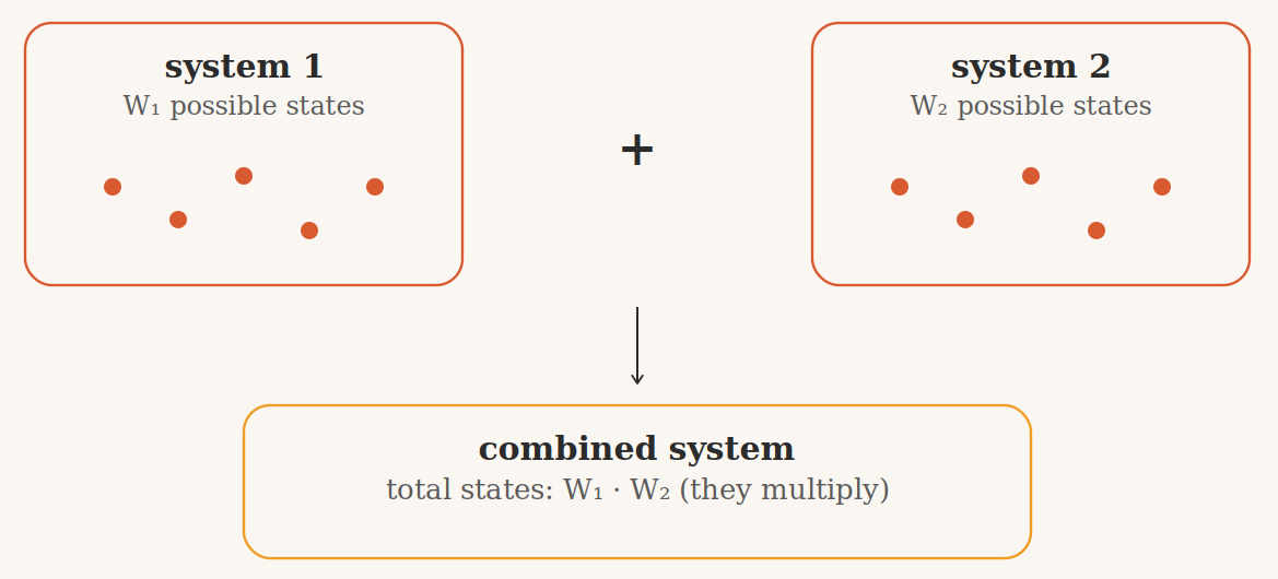

A continuous function with these properties does exist, and it is called the logarithm. It also has a second very interesting property: the logarithm brings very small values onto a manageable scale ($\log(10^{-300})$ is simply $-300 \cdot \log(10)$, an ordinary number). And in this case we’ll need it, because the probabilities of independent events multiply, and the product of many small numbers quickly becomes a number so small it’s unmanageable.

So Boltzmann defines:

$$ S = k_B \ln(W) $$

and calls this quantity $S$ entropy.

a word on $k_B$: the constant $k_B$ does not come from the derivation just made. The additivity constraint only tells us that the function must be a logarithm, not which factor to multiply it by. That factor is a pure choice of units.

How much information do you read in a cup of coffee?

Moving further along in history, and more precisely to 1948, Claude Elwood Shannon (the father of modern information theory), without making anyone angry this time, posed a different problem: how much uncertainty does a probability distribution $\{p_1, \ldots, p_K\}$ over $K$ possible events contain?

Let’s start with the single occurrence. Let’s call surprise the amount of information we gain from seeing an event of probability $p$ happen: an almost certain event tells us almost nothing (low surprise), an extremely rare event tells us a great deal (high surprise). And here Boltzmann’s constraint comes back exactly. If I observe two independent events, their probabilities multiply ($p_1 \cdot p_2$), but the surprise I draw from them has to add up: seeing two independent things informs me as much as the first plus the second. So we need a function $s$ such that

$$ s(p_1 \cdot p_2) = s(p_1) + s(p_2) $$

It is the very same functional equation as before, and its only continuous solution is once again the logarithm. Since probabilities lie between 0 and 1 (and their logarithm is negative), to obtain a positive surprise we put in a minus sign: $s(p) = -\log(p)$.

At this point the uncertainty of an entire distribution is simply the expected surprise, that is, the average of the surprises weighted by the probabilities with which each event occurs:

$$ H = \sum_{k=1}^{K} p_k \cdot s(p_k) = - \sum_{k=1}^{K} p_k \log(p_k) $$

This is Shannon’s Entropy. It doesn’t measure physical “disorder”, but the expected amount of surprise in a distribution. The same derivation as Boltzmann, the same logarithm, applied however to surprise instead of to the number of states.

Let’s go back to my grandfather’s cup of coffee and imagine a simplified little model with two compartments of equal capacity: the cup and the environment immediately around it (the table, the air). Let’s ask ourselves a question: if I were to pick a unit of heat at random, in which of the two compartments would I find it?

Just after the coffee is poured, the answer is easy. The heat is still almost entirely in the cup, because it hasn’t yet had time to spread. The probability distribution over the two compartments is almost entirely concentrated on one option: $p_{\text{cup}} \approx 1$, $p_{\text{table}} \approx 0$. My uncertainty is extremely low, I’m almost certain of the answer, so $H$ is almost zero.

If my grandfather gets distracted for long enough, the two compartments reach the same temperature. The same question becomes much harder, since by now the heat has been shared between the two. At this point the two probabilities get close, $p_{\text{cup}} \approx p_{\text{table}} \approx 0.5$, and I no longer have any clue for choosing between the two options. Now my uncertainty is maximal, so $H$ is maximal.

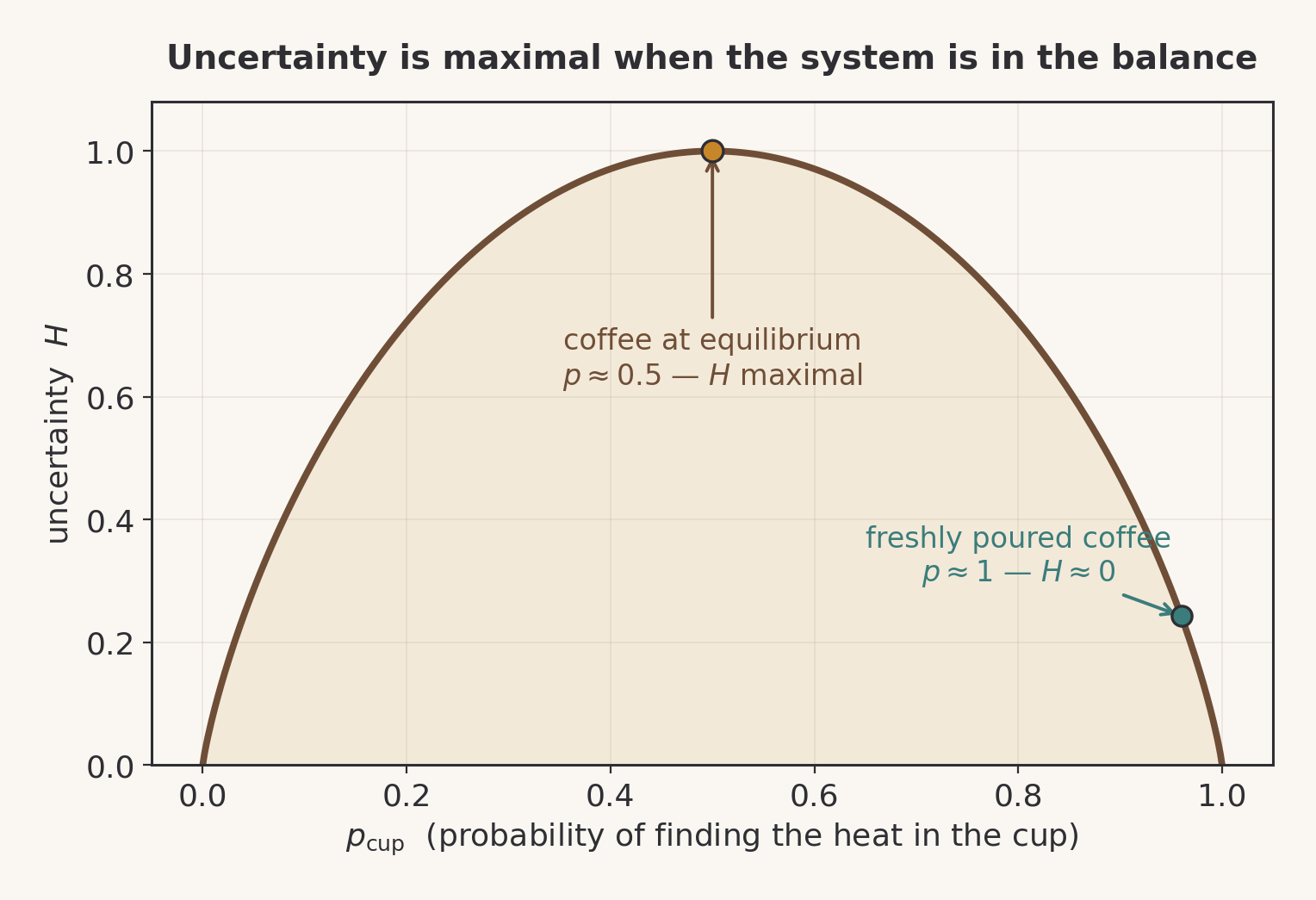
This two-outcome question, cup or table, has exactly the same structure as the question the neural network will ask later on: cat or dog, class 1, class 2 or class 3. In both cases $H$ measures how much the system is poised between the available options.

Coffee is good for your neurons

I don’t know whether it’s true, but my grandfather used to tell me often before an exam: “have a coffee before you start, it’s good for the brain”. But since it was him who told me, and since I like my coffee long and lukewarm, I’ll make up for it by proving it mathematically.

So, where did we leave off with neural networks? We had a model $\boldsymbol{f(x, \theta)}$ and a final layer of the network producing $K$ arbitrary numbers:

$$ \boldsymbol{f(x, \theta)} = \{f_1, f_2, \ldots, f_K\} \in \mathbb{R}^K $$

like the cup of coffee, before the direction of the heat flow is observed, the model hasn’t chosen yet. It lives in a space of values of any kind. The probability isn’t described in any way.

To turn them into a valid probability distribution over $K$ classes, two conditions are needed, both dictated by the very meaning of probability:

• no value can be negative, because it makes no sense to say that an event has a “minus 20%” probability of happening

• the values must add up to exactly 1, because I’m certain that only one of the $K$ possible outcomes can occur, no more and no less.

A function that satisfies both conditions is the softmax, applied to the raw outputs $z_k = f_k$ of the network:

$$ \lambda_k = \text{softmax}_k(\mathbf{z}) = \frac{e^{z_k}}{\sum_{k'=1}^{K} e^{z_{k'}}} $$

Where:

• the exponential $e^{z_k}$ is always positive, whatever $z_k$ may be, which guarantees the first condition

• by dividing by the sum of all the exponentials, we obtain $\sum_k \lambda_k = 1$ and the second condition is satisfied too.

And here “exactly like” is not a figure of speech. It’s the point I’d like to pause on for a moment, because in my opinion it’s the most beautiful thing in this whole story.

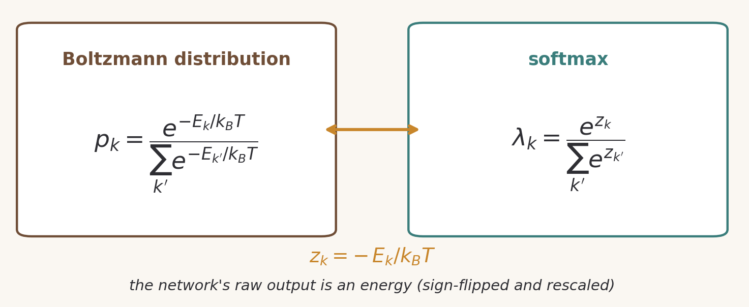
Besides entropy, there is another formula that bears Boltzmann’s name: the Boltzmann distribution, which gives the probability of finding a physical system in state $k$, with energy $E_k$, at temperature $T$:

$$ p_k = \frac{e^{-E_k / k_B T}}{\sum_{k'} e^{-E_{k'} / k_B T}} $$

Let’s place it under the softmax and look at them together. It’s the very same form. The only difference is what sits in the exponent: where Boltzmann has $-E_k / k_B T$, the network has $z_k$. For the rest, it’s not an analogy, it’s the same equation.

Put another way: the raw output of the network is an energy, with its sign and scale changed. A high value corresponds to a low energy, and in physics low-energy states are the most probable. The network, without knowing it, assigns each class an energy level and then lets Boltzmann statistics decide how probable it is. The denominator too (the sum over all the states) has a name in thermodynamics, the partition function, and we’ll meet it again shortly, disguised as $\log \sum_{k'} e^{f_{k'}}$.

So, claiming that the model, like the cup of coffee, lives in a distribution defined over all the possible states before observation pins one of them down, doesn’t mean borrowing an image from physics at random, it means we are describing substantially the same equation.

the temperature of the coffee: the resemblance can be carried all the way through. If in the softmax we divide the exponent by a parameter $T$:

$$ \lambda_k = e^{z_k / T} / \sum_{k'} e^{z_{k'} / T} $$

we literally recover Boltzmann’s temperature, and with it my grandfather’s cup. With high $T$ the exponents flatten out, the probabilities get closer and the distribution tends toward the uniform: maximal uncertainty, maximal $H$, the coffee now at equilibrium. With $T \to 0$ a single state dominates and the distribution collapses onto a single class: it’s the freshly poured coffee, and it’s exactly the $\arg\max$ we’ll use in inference. Cooling the softmax and cooling the coffee are the same operation.

Probably this is a mistake

Boltzmann had found the way to measure the “disorder” of a physical system. Shannon had found the way to measure the uncertainty of a probability distribution. One last question remains: how do we measure how wrong the distribution predicted by the model is, with respect to the expected result?

Let’s start from something we settled in the articles on neural networks: for every training example $i$ we have the expected result $y_i$. We can describe this last one as a probability distribution even though there’s nothing genuinely uncertain about it. In the sense that, given the set of expected results, we can directly assign $1$ to the correct result and $0$ to the rest, $y_i = \{0,1,0,\ldots, 0\}$. This is a distribution concentrated entirely at a single point, which in statistics is called degenerate.

Let’s take a practical example: we’re training an animal recognition model, the distribution of our ground truth could be represented like this:

$$ \begin{align*} \boldsymbol{y}_1 &= \{ 1, 0, 0, 0, \ldots \} = \text{cat} \\ \boldsymbol{y}_2 &= \{ 0, 1, 0, 0, \ldots \} = \text{dog}\\ \boldsymbol{y}_3 &= \{ 0, 0, 1, 0, \ldots \} =\text{bird}\\ \boldsymbol{y}_4 &= \{ 0, 0, 0, 1, \ldots \} =\text{fish}\\ y_n &= \ldots \ \ \ = \ldots \end{align*} $$

Good, now we can have two distributions to compare over the same $K$ classes: the one generated by the model, $\{\lambda_k\}$, and this distribution in which every element is concentrated on the right class. How different are they?

Shannon had measured the uncertainty of a single distribution with $H = -\sum_k p_k \log p_k$. To measure the discrepancy between two distributions we use the same idea. We compute the logarithm of the model’s distribution and compare the result with the probabilities of the ideal distribution. Since the ideal distribution has probability 1 only on class $y_i$ and 0 on all the others, only a single term survives in the sum, and it is given by the logarithm of the probability the model assigns to precisely the correct class.

This quantity is called cross-entropy, and in its general form it is written:

$$ H(p, q) = -\sum_{k=1}^{K} p_k \log q_k $$

where $p$ is the ideal distribution (the ground truth) and $q = \{\lambda_k\}$ the one predicted by the model.

Certain, dead certain, actually probable

The aphorism is by Ennio Flaiano, who was not a mathematician but an Italian journalist and intellectual whose irony, now more than ever, deserves to be cultivated.

Having reached this point, there’s an important issue I’d like to point out: in the article on neural networks we defined error in terms of distance, whereas in the previous section we talked about “discrepancy” between probability distributions.

So before formally describing the probability we want to maximize, it’s worth pausing for a moment on what that probability means.

What is the probability that it rains? The answer changes radically if I add a piece of information: what is the probability that it rains, knowing that the sky is already covered with black clouds?

Probability doesn’t live on its own. It is always the probability of something, computed knowing something else. This “knowing” is exactly what we meant with Boltzmann, even if we didn’t make it explicit. Changing the energy changes the number of accessible states, and so changes the entire probability distribution over which Boltzmann measured disorder.

In our case, instead, that “knowing” is the output of the network. Changing the parameters $\theta$ changes what the network computes and therefore changes the entire distribution over the classes. We aren’t asking “how probable is the right class” in absolute terms, but “how probable is the right class, given what the network has computed from the input”.

This is the probability we’re talking about:

$$ P(y_i \mid f(x_i, \theta)) $$

We can read the formula as: the (conditional) probability of the correct answer $y_i$, knowing what the model $f$ computed starting from the input $x_i$ with the parameters $\theta$. In the second part of the article on neural networks we talked about a shift in point of view between inputs and parameters. The same thing happens here: the parameters $\theta$ are what we want to “adjust” during training. The same network, with the same weights, has to assign the correct probability to every different input presented to it.

This is the probability we obtain by comparing each result with the degenerate distribution of the ground truth.

The folds of definitely maybe

So we’ve arrived at a part I care about a great deal, because in my opinion it lets us glimpse the folds where the true complexity of deep learning is hidden.

Let’s imagine a gas in a closed and isolated box, where no energy enters or leaves. This means the total energy of the gas is fixed.

The molecules, however, move continuously and exchange energy among themselves. At every instant the total energy is the same, but it can be distributed in different ways among the molecules.

Probability, then, doesn’t concern “any possible state”, but only those in which the sum of the molecules’ energies stays equal to the fixed value. All the other states are excluded because they would violate the constraint.

In other words: the gas can be in many different microstates, but only those compatible with the total energy really count. Probability is never absolute, it is always conditional on what we hold fixed (here, the energy). It’s the same “knowing” as the rain and the black clouds, and it’s the same one we wrote a moment ago in $P(y_i \mid f(x_i, \theta))$: the model’s distribution isn’t “just any” distribution, it’s the one conditioned on what the network has computed from the input. The gas constrained by its energy and the model constrained by its output are two conditional distributions, and this is the real point of contact.

With this settled, the next step consists in maximizing the probability the model assigns to the correct class for each example in the dataset:

$$ \hat{\theta} = \underset{\theta}{\arg\max} \prod_{i=1}^{I} P(y_i \mid f(x_i, \theta)) $$

The product form comes from the assumption that the examples are independent and identically distributed (i.i.d.), which lets us factorize the joint probability as the product of the probabilities of the individual samples. But for the same reasons as Boltzmann and Shannon, the measure has to be additive. So we apply the logarithm, and we can do so without consequences because it is a monotonically increasing function (it doesn’t move the position of the optimal points, but turns the product into a sum). The point that maximizes the product is exactly the one that maximizes the sum of the logarithms. It’s a property that will come in handy with gradient descent.

$$ \hat{\theta} = \underset{\theta}{\arg\max} \sum_{i=1}^{I} \log P(y_i \mid f(x_i, \theta)) $$

I’d say we’re there, we’ve given an answer to the request to formalize the error. But our problem is one of minimization, and there’s an $\arg\max$ in the formula that clashes quite a bit.

No problem, changing the sign of a function doesn’t change where its extreme points are, it only swaps them. So the point that maximizes a sum is exactly the same point that minimizes that sum with its sign changed. It follows that we can write the same $\hat{\theta}$ as before in a completely equivalent way, as a minimization problem:

$$ \hat{\theta} = \underset{\theta}{\arg\min} \left[ -\sum_{i=1}^{I} \log P(y_i \mid f(x_i, \theta)) \right] $$

It’s time to give a name to the expression in brackets: cross-entropy loss. And from the name you should grasp its role within a neural network, being fundamentally a function belonging to the family of loss functions.

$$ L(\theta) = -\sum_{i=1}^{I} \log P(y_i \mid f(x_i, \theta)) $$

So we could rewrite our minimization problem as follows:

$$ \hat{\theta} = \underset{\theta}{\arg\min} \; L(\theta) $$

Here too, the penalty is logarithmic for the same structural reason as Boltzmann and Shannon. The asymmetry is built into the form: if the model assigned high probability to the right class, $-\log P$ is small. If it was very confident and got it wrong, $-\log P$ explodes.

Being certain and being wrong costs much more than being uncertain and being wrong, not by design choice, but because of the geometry of the logarithm near the extremes.

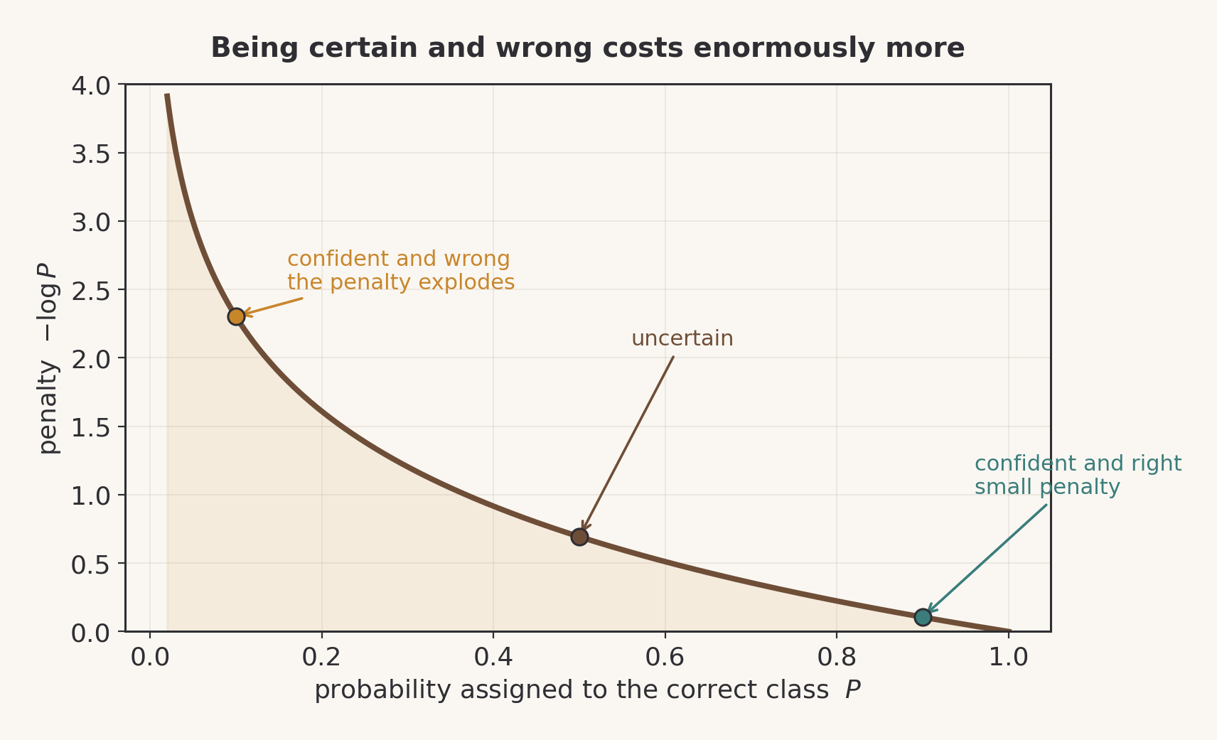
brief didactic note:

By substituting the softmax explicitly into the loss, we obtain a computationally more tractable form.

$$L(\theta) = -\sum_{i=1}^{I} \left( f_{y_i}(x_i, \theta) - \log \sum_{k'=1}^{K} e^{f_{k'}(x_i, \theta)} \right)$$

The first term rewards the output corresponding to the right class. The second penalizes all the outputs. This form is also numerically more stable than explicitly computing the softmax and then taking its logarithm, and it’s generally the formula you’ll find in various textbooks.

A gradient of probability

What changes in backpropagation? The structure is substantially identical. The only thing that changes is the error signal at the output ($\delta^L$), which is now computed starting from the cross-entropy instead of from the MSE. Everything else (gradients, weight updates, gradient descent) works exactly as described in Part 2:

$$ (\theta - \eta \cdot \nabla_\theta \mathcal{L}) \rightarrow \theta $$

There is, however, one peculiarity worth describing. Putting softmax and cross-entropy together, the derivative of the loss with respect to the raw outputs simplifies until it disappears into a single line.

$$ \delta_k^L = \lambda_k - y_k $$

The signal that travels back through the network is simply the difference between the probability the model assigned and the one it should have assigned. Nothing else. It’s one of the most elegant formulas in deep learning, and it’s no accident at all. Softmax and cross-entropy were chosen partly because, together, they produce exactly this simplification.

There’s then another particularly interesting aspect. The loss:

$$ L = -\log P $$

can grow without any limit when the model gets it wrong with great confidence. If the correct class is assigned a probability ever closer to zero, the penalty becomes ever more severe and tends to infinity. One might then expect the gradient too to explode because of overly large gradients (it’s one of the various effects of training gone wrong, we’ll talk about it). In reality the opposite happens.

Thanks to the mathematical structure of the softmax, the terms that would tend to make the derivative diverge cancel each other out exactly.

So the final result remains:

$$ \lambda_k - y_k, $$

a value that can never leave the interval between $-1$ and $1$.

This is an extremely useful property. The loss function (or cost function) can draw a drastic distinction between a moderate error and an error committed with absolute confidence, increasing the penalty indefinitely. At the same time, the learning signal stays controlled and numerically stable.

In other words, the model is punished ever more harshly for the most serious errors, but without the optimization process being overwhelmed by out-of-scale gradients. It’s one of the reasons the softmax and cross-entropy pairing has become the standard for multiclass classification problems.

Eeny, meeny, miny, moe

Once the network is trained, inference is the moment in which the probability distribution $\{\lambda_k\}$ turns into a decision.

Now, careful, this might sound like a nursery rhyme. If during the minimization phase we had to find the minimum error, now it’s the other way around, we have to take the class with the maximum probability:

$$ \hat{y} = \underset{k}{\arg\max} \; \lambda_k = \underset{k}{\arg\max} \; f_k(x, \hat{\theta}) $$

The softmax doesn’t change the relative order of the values (the exponential is monotonic), so we can look directly at the network’s output without applying it. The distribution stays there, intact, with all its uncertainty.

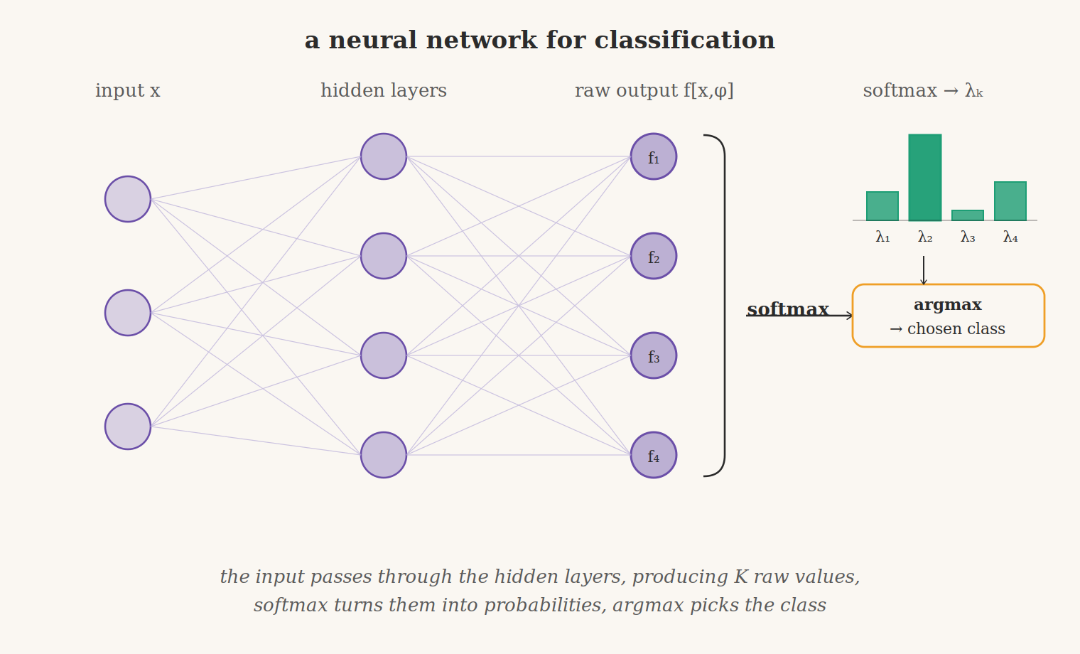
It’s only at the moment a response is needed that a single one is extracted from it. Exactly like the cup of coffee, it doesn’t stop obeying statistics just because we observe one direction for the flow of heat.

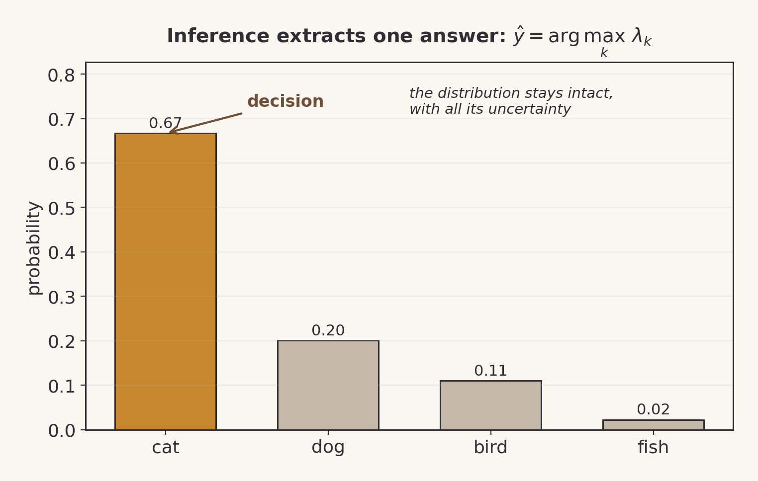
The underlying probability distribution doesn’t disappear, it simply stops being of use to us at the moment of decision.

The network becomes a system able to give a result with the right dose of “uncertainty” rather than “certainty”. You could say it “learns to spread its bets well”. Acceptable and negligible, we’re always back there.

binary classification: we’ve described how multiclass classification works, but for binary classification ($K = 2$) not much changes. The softmax reduces to a simpler form called the logistic sigmoid:

$$ \sigma(z) = \frac{1}{1 + e^{-z}} > $$

This function essentially squashes a single real value into the interval $[0, 1]$, directly interpretable as the probability that the example belongs to class 1. The sigmoid is the special case, the softmax is the general case.

Key terms

• Softmax: a function that transforms $K$ arbitrary real values into a valid probability distribution. Guarantees non-negative values that sum to exactly 1.
• Temperature (in the softmax): parameter $T$ controlling how “flat” the distribution is. High temperature: uniform distribution, maximal uncertainty. Temperature approaching zero: distribution collapsed onto a single class.
• Degenerate distribution: a probability distribution concentrated entirely on a single event. Used to represent the ground truth in classification.
• Conditional probability: the probability of an event computed knowing that another event has occurred. Notation: $P(y_i \mid f(x_i, \theta))$.
• Cross-entropy: measures the discrepancy between two probability distributions. In classification it compares the distribution predicted by the model with the ground truth.
• Cross-entropy loss: cost function for classification, defined as $L(\theta) = -\sum_i \log P(y_i \mid f(x_i, \theta))$. Penalises errors made with high confidence more harshly.
• Argmax: operation that returns the index of the maximum value in a set. Used in inference to select the most probable class.
• Inference: the phase in which the trained network produces a prediction on new data, selecting the class with the highest probability.
• Logistic sigmoid: special case of the softmax for binary classification ($K=2$). Defined as $\sigma(z) = 1/(1+e^{-z})$, maps a real value into the interval $[0,1]$.