It's all about Origami (Part 2)

(How to fold paper while walking down a mountain and, in the meantime, understand how to train neural networks)

I already said I am not particularly good at origami, and those times I do try, the first version is certainly never the right one.

We saw how origami take shape through several steps in which each layer depends on the previous one, so once we reach the last fold, what do we do? We choose a method capable of quantifying the error we make every time we finish our synthesis process.

I generally use, as my method, presenting the result to my son.

And so it goes:

• the first version looks like a Gremlin.

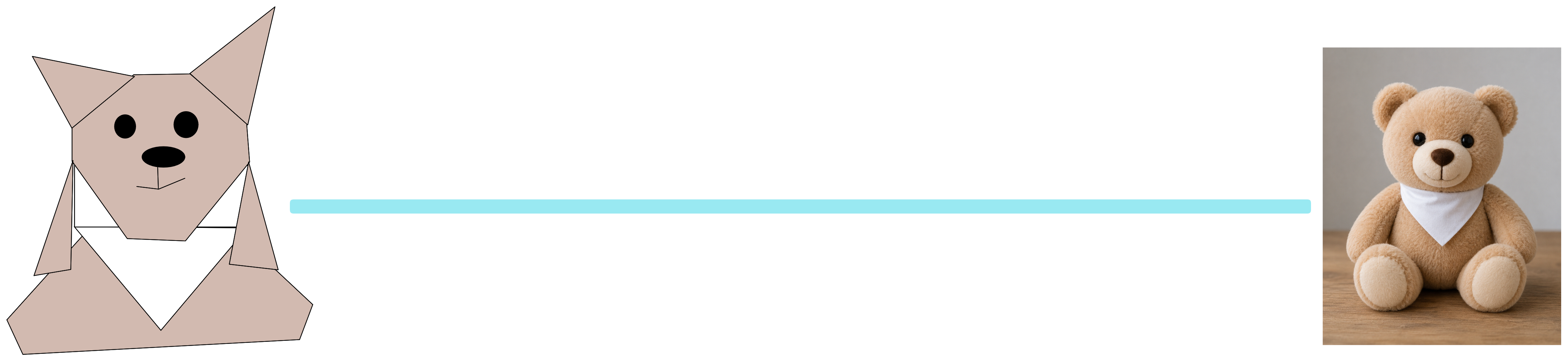
• the second looks like a dog

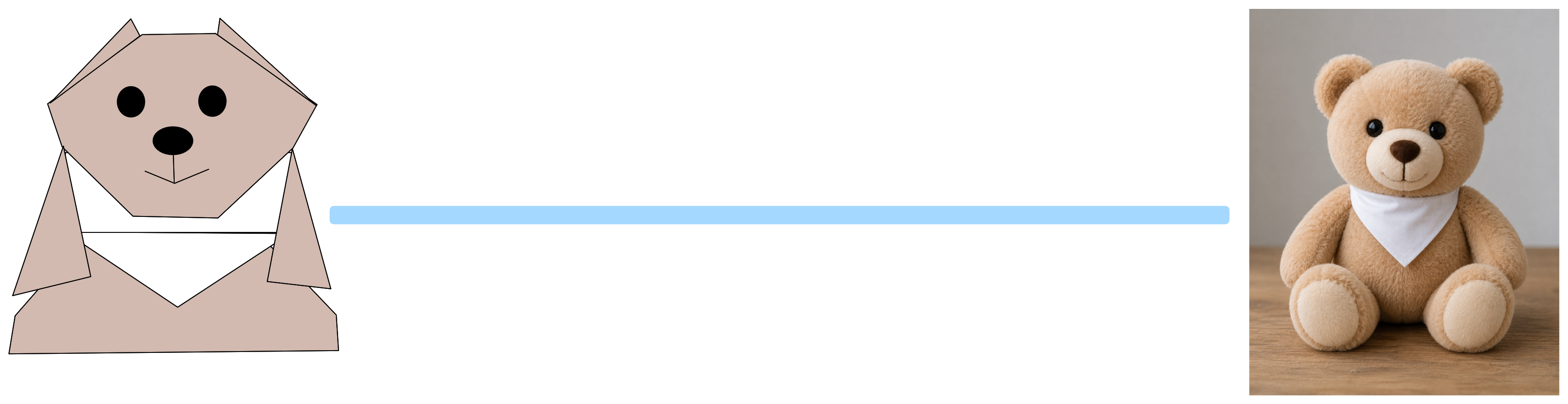
• the third maybe looks like a teddy bear

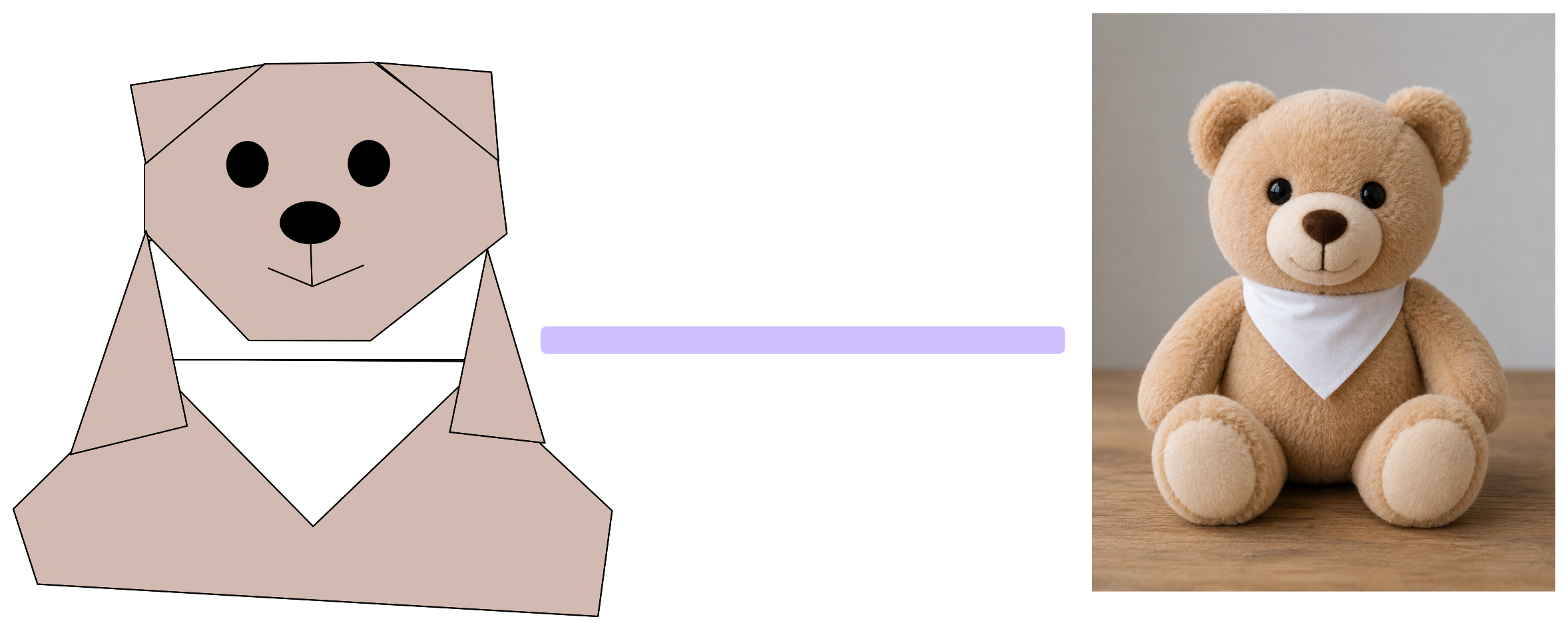
• on the fourth attempt we finally got it

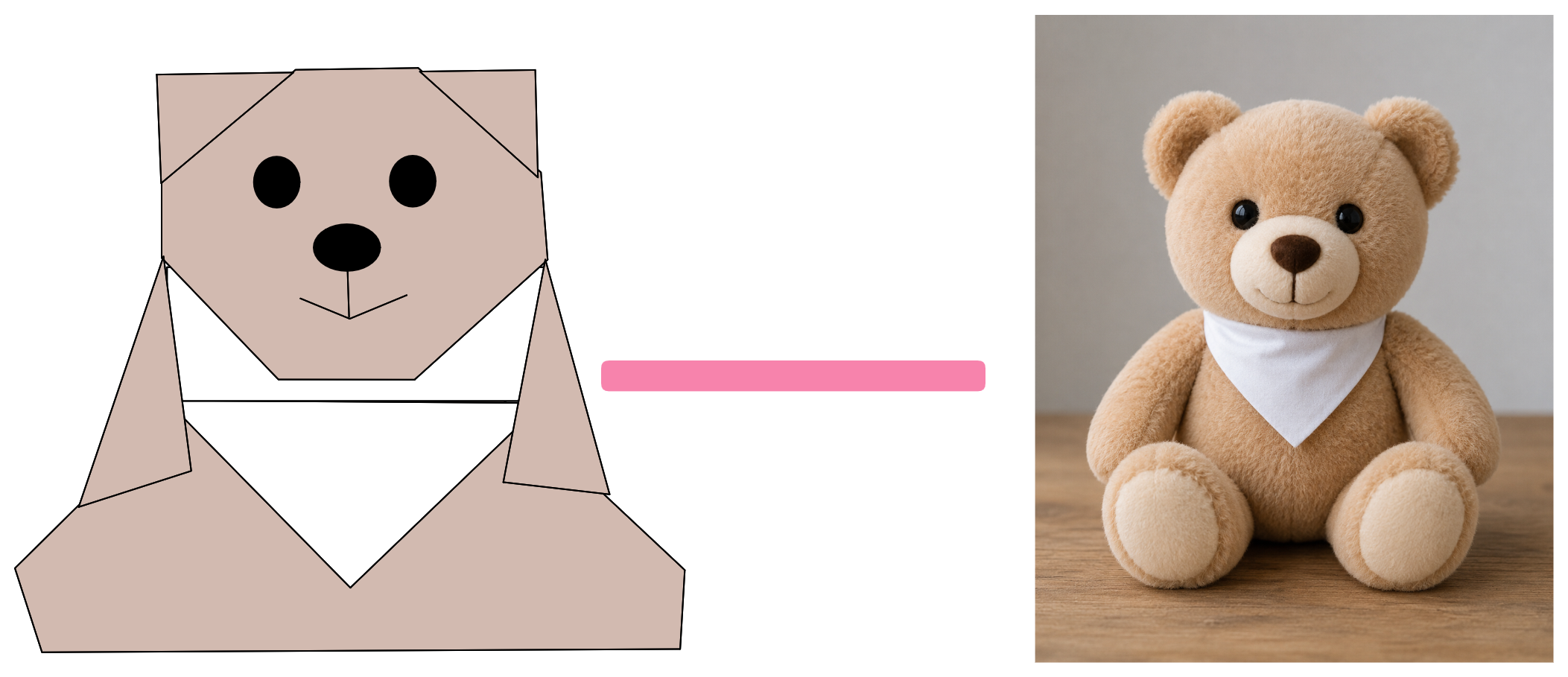
Let us try to write a recipe for the perfect origami:

• I study what to represent, moving from the general shape to the details, trying to figure out how to synthesise everything

• the folds of the paper, the point at which to place them, are the parameters of my process. By varying their position I can create a series of progressive steps in which each layer is influenced by the previous one.

• I carry out a series of attempts in which:

  • I try to quantify the error that determines the distance from the expected result
  • I try to understand how to minimise the error across all steps by analysing how this error propagates through the folds
  • I repeat until I reach an acceptable approximation with negligible error.

Natura non facit saltus (nature does not make jumps)

With this expression the mathematician Leibniz recalled the idea that changes occur through a succession of continuous steps. Between one state and another there is not necessarily a sharp break, but a series of progressive transformations.

This will strike many as a purely philosophical quotation, but it has had a profound influence on the way mathematics describes change and still represents one of the conceptual foundations of modern science. But aside from this clarification, I also find it an excellent vantage point from which to begin observing our error minimisation problem.

It is not just a numerical question: in the first part of this article we put together a composition of functions whose purpose is to model a series of “changes” aimed at reaching an ideal shape.

But how can we describe this change and quantify it?

Quantifying the gap

If in comparing our origami the measure remains a visual factor, for the curve introduced in the first part we will need to find a decidedly more reliable tool.

Let us reason through it step by step.

• We have a model $\hat{y} = f(x, \theta)$ where $\theta$ represents the set of all parameters:

  $$\theta = \left\{\alpha_{kj}^{l},\ \beta_k^{l},\ \phi_0,\ \phi_k\right\}$$

• We start by comparing, point by point, the results predicted by the model $\hat{y}_i$ with the real values of the dataset $y_i$.

  This is a very simple operation; it suffices to calculate the difference between the two values:

  $$ e_i = (y_i - \hat{y}_i)^2 $$

  Here the squaring has two jobs: to weigh large errors more heavily and to ignore the sign, making the result always positive.

• So now we have a set of values composed of $N$ residuals depending on how large our dataset is.

  $$ \boldsymbol{e} = \{ (y_1 - \hat{y}_1)^2, (y_2 - \hat{y}_2)^2, \ldots, (y_i - \hat{y}_i)^2 \} $$

• We need a single number that summarises how much we are getting wrong, and what better way to obtain it than the average of the residuals. So let us add them all up and divide by their count.

  $$ L(\boldsymbol{\theta}) = \frac{1}{N} \sum_{i=1}^{N} \left( y_i - \hat y_i \right)^2 $$

  We will call loss function $L(\boldsymbol{\theta})$ that family of functions capable of quantifying the error between the predicted values and the real values (called ground truth).

Changing point of view

We have given an idea of distance for the origami; now let us represent the error just as we have formalised it for the curve.

Now, let us stop for a moment and ask ourselves a question: if we were to bring all the points of the origami onto the image of the teddy bear, would it be useful for quantifying the error?

The answer is no.

Until now this has been a question that was always hinted at but that the loss function brings to the surface clearly. If I want to reach the smallest possible error I must change point of view; I must understand what happens inside the folds.

It is a reversal of roles we are not used to from school: what was a variable (the $x$) becomes a constant, and what seemed a fixed coefficient (the parameters $\alpha, \beta, \dots$) becomes the variable. With it, the space in which we look also changes: no longer the data space, but the parameter space.

Let us set aside our curve for a moment; it is worth fixing this concept by looking at what happens with a single parameter $\alpha$ and a generic line $y = x \cdot \alpha$.

Looking at the images, on the left we see the space generated by the data while on the right the space generated by the parameter $\alpha$ and by the loss function $L(\theta)$. Where $\boldsymbol{\theta} = \{\alpha\}$

Let us try starting from a value of $\alpha$ chosen at random, but within a range of values consistent with my data.

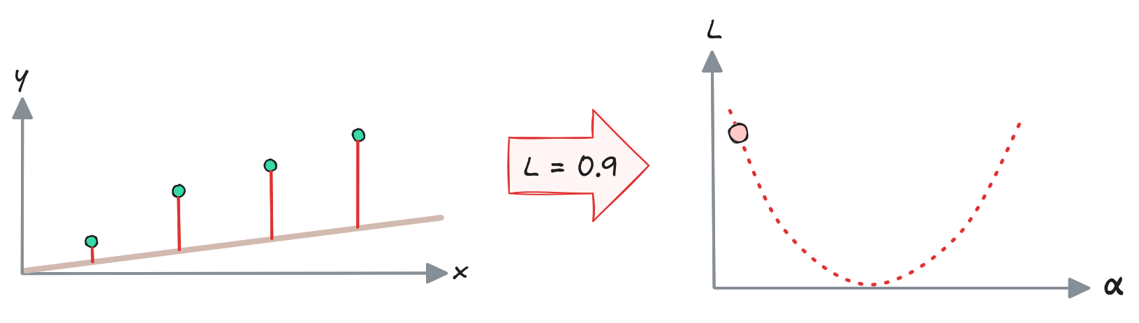
It is clear that the chosen value is rather low; the prediction line is well below the target points.

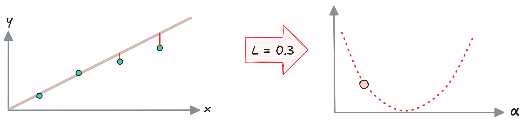
Now the slope seems larger than necessary. The prediction level has improved, the error has decreased, but we are decidedly not there yet.

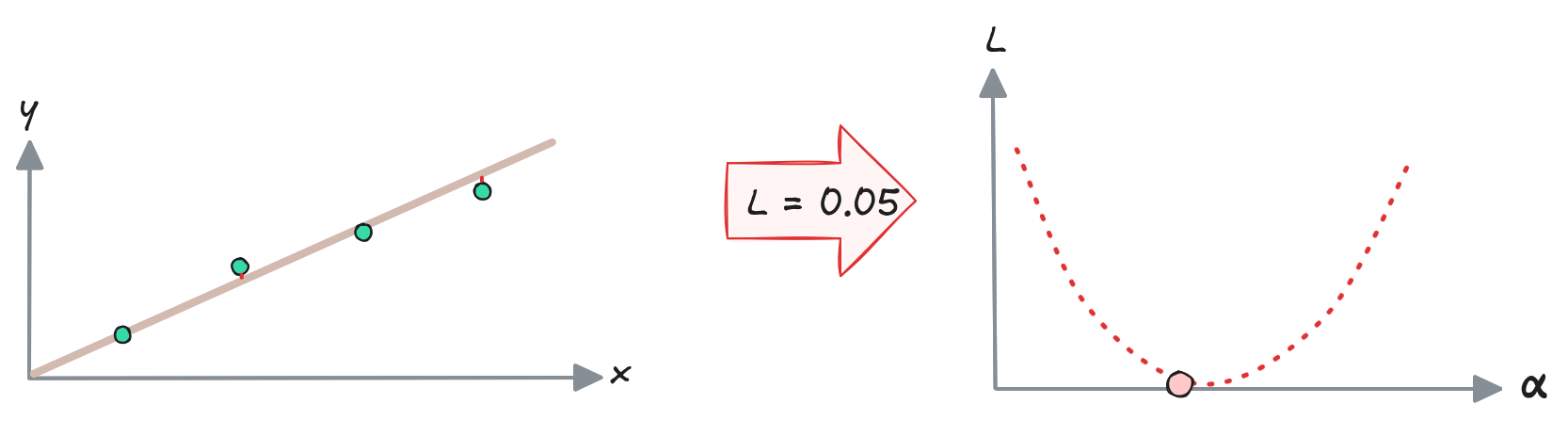
This last attempt we can say has gone well; we have found the value of $\alpha$ that produces a sufficient loss value.

Let us put in order what we have seen:

• finding the right parameters means finding the set of values $\theta$ that minimises $L(\theta)$.
• the more the results of the loss function tend towards zero, the closer the model gets to generalising the shape of the target data.
• the loss function has a geometry of its own where one can see how the search for the minimum essentially amounts to traversing it towards the lowest part (absolute minimum).

Good. But now let us look again for a moment at what we did for the origami: however extremely empirical, we did find a method. We had a judge and it was possible to quantify our errors because between the ears of a Gremlin and those of a Bear we can grasp some kind of “distance” and reduce it. With the curve the judge is the loss function, and up to this point I have queried it by eye: this $\alpha$ is too low, that one too steep, this last one, we are almost there.

Let us continue reasoning on the single parameter $\alpha$; it is easier to work with and the leap towards a richer set $\boldsymbol{\theta}$ will come more smoothly.

If you recall what was said in the first part, acting on the parameter $\alpha$ essentially means moving the line about one end so as to rotate it just enough to get a good approximation. Let us also reverse the point of view here:

• which way should I move along the trajectory traced by the loss function?
• by how much?

Getting closer until the jump vanishes

If I do not want to jump, then I do not leap to the minimum; I take an infinitely small step.

Let us call $\mathrm{d}\alpha$ this step so tiny as to be smaller than any positive number imaginable. But be careful: it is not zero. Recall that we are in the parameter space, so as $\alpha$ varies the loss will respond with an equally tiny shift that we will call $\mathrm{d} L$.

If we were to place a lens powerful enough on the curve right at that point, we would see the curve become a straight line and we could observe its slope, noting that it is nothing other than the ratio between the two variations: $\frac{\mathrm{d} L}{\mathrm{d} \alpha}$

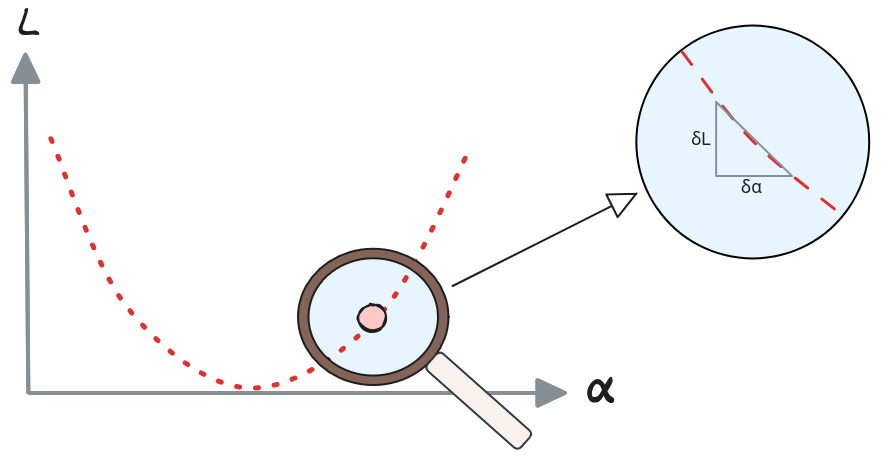
We are talking about an operation that in mathematics has a very precise name: the derivative.

H. Jerome Keisler, in his book Elementary Calculus: An Infinitesimal Approach (1976), builds all of calculus precisely on infinitesimals, through a wonderful non-standard approach. Imagine placing on the curve $L(\alpha)$ an infinite-magnification lens. This is the didactic device with which Keisler makes visible numbers that are infinitely close to one another.

The more you magnify, the more the curvature vanishes. At infinite magnification that arc of curve becomes indistinguishable from a straight line.

The derivative is simply the slope of that local straight line. Nothing more. The curve was daunting as a whole (made of all the folds, of all the parameters) but seen closely enough, around a single point, it is just a line with a certain inclination.

At this point we can write it down. We take the position of the loss $L(\alpha)$ (for a given $\alpha$) and that after an infinitesimal step, $L(\alpha + d\alpha)$. Their difference, divided by the step, is precisely the slope of the straight line that the magnifying lens showed us.

$$ \frac{\mathrm{d} L}{\mathrm{d} \alpha} = \frac{L(\alpha + \mathrm{d} \alpha) - L(\alpha)}{\mathrm{d} \alpha} $$

And the result is a single, exact number, and it tells us everything we needed:

• its sign tells us which way the curve rises. If the slope is positive, to the right it goes up; to go down one must go left. And vice versa. To minimise, one always moves in the direction opposite to the sign.
• its absolute value tells us how steep the slope is. The larger it is, the farther we are from the bottom and the bolder the step can be. Near the minimum it flattens towards zero and the steps become small on their own.

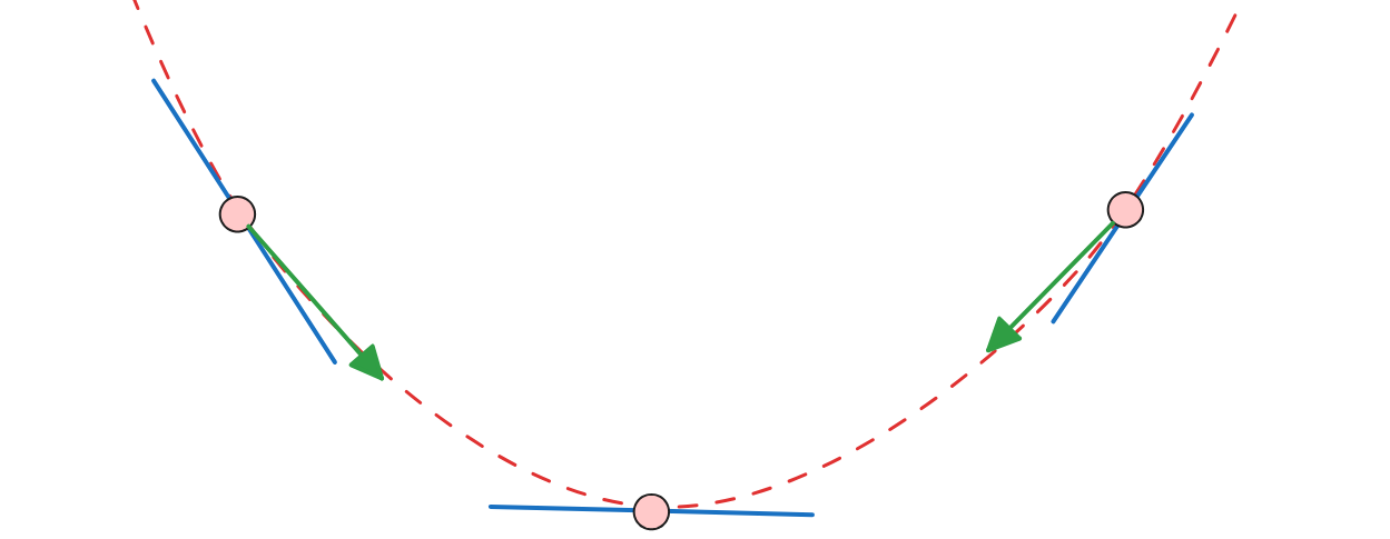
It is exactly the logic with which we tackled the folds of the origami. At each attempt one looks at the direction from which one is moving away from the right shape and “quantifies” the correction. The derivative gives us the same indication, but written as a number.

A gradient of possibilities

With only the parameter $\alpha$ the parameter space is small and insufficient. But before expanding the set $\theta$ towards the representation of the neural network seen in the first part, I would like to make one thing clear: we have understood which tools are appropriate and how to use them.

Let us take one step at a time: we go from one parameter to two parameters, $\boldsymbol{\theta}= \{\alpha, \beta\}$. The space expands and it starts to become more complicated to have an effective visualisation strategy. With a single parameter the derivative is just “this way or that way”, but with two the loss is a surface.

Let us try to visualise this surface as contour lines, in this case represented as a series of concentric rings. The farther outward you go, the higher the loss; moving towards the centre we aim at useful minimisation values.

With a single parameter we have one derivative. But our $\theta$ in reality has lots of parameters:

$$ \theta = \{\alpha_1, \beta_1, \ldots, \alpha_n, \beta_n, \phi_0, \phi_1, \ldots, \phi_n \} $$

consequently we will have a derivative for each one of them.

That set of slopes, one per direction, has a name: it is called the gradient, and it is the compass with which to orient oneself in the parameter space.

Increasing our space to include the intercept parameter $\beta$ as well, we can therefore write:

$$ \nabla L(\theta) = \left( \frac{\partial L}{\partial \alpha}, \frac{\partial L}{\partial \beta} \right) $$

where the $\mathrm{d}$ becomes $\partial$ and the individual derivatives are called partial derivatives.

We said that the objective is to minimise the loss and therefore one must “traverse the geometry of the loss downward”. And if we consider that the gradient points uphill, the solution then becomes a precise operation: gradient descent, $-\nabla$.

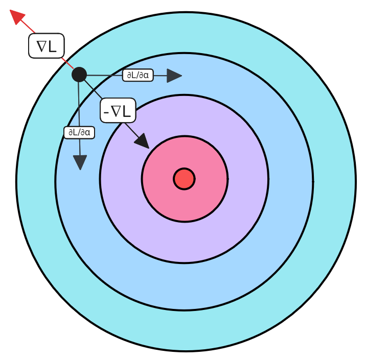
Before moving on, however, I would like the difference between derivative and gradient and where we have arrived to be well understood. I introduced this last term almost reducing it to a simple change of vocabulary, so it is worth clarifying.

If I walk on a tightrope, I can move in only two directions: forward or backward. At every point of the rope, the derivative indicates its exact slope at that point. In other words, the derivative measures how quickly the height changes as I advance along the rope: if it is positive I am climbing, if it is negative I am descending, and the larger its absolute value, the steeper the ascent or descent.

If instead I find myself on the side of a hill, I can move in multiple directions. To understand the shape of the terrain, I can measure the slope along two fundamental directions, for example east-west and north-south. These slopes are the partial derivatives. By putting the partial derivatives together I obtain the gradient, a vector that indicates the direction of steepest ascent. If I want to reach the lowest point of the valley, instead of following the gradient I move in the opposite direction: this is the principle of gradient descent.

Now we can present the two formulas for $\alpha$ and $\beta$:

• With respect to the slope $\alpha$:

  $$ \frac{\partial L}{\partial \alpha} = \frac{2}{N} \sum_{i=1}^{N} x_i (\hat y_i - y_i) $$

• With respect to the intercept $\beta$:

  $$ \frac{\partial L}{\partial \beta} = \frac{2}{N} \sum_{i=1}^{N} (\hat y_i - y_i) $$

As one can see, these are extremely simple formulas.

Uphill the lungs, downhill the eyes

I do not remember the origin of the saying; a friend of mine used to repeat it often during our mountain walks when I would quicken my pace on the descent. Of course, it would have been better to add to the saying: “and at the summit, do not bring the wine”. But the point is another.

That saying, in its simplicity, describes something very concrete: uphill the body forces you to follow your breathing, while downhill it is your sight that sets the pace, because the danger is not fatigue but the wrong foothold.

From a completely different quarter, in the 1950s and ’60s, a similar issue was encountered in minimum-search problems. The first approaches tended to move rigidly or “by leaps” towards an estimated solution. They basically all failed for two main reasons:

1. Oscillations and instability (overshooting) Without control over the magnitude of the updates, corrections can become too aggressive and make gradient descent “bounce” past the optimal solution.
2. Complex error surfaces In real problems the error function is neither simple nor smooth. It presents many variations and local minima.

A solution was found by adding a new parameter: the learning rate. To reduce the loss we move in the direction opposite to the gradient, by a step proportional to the learning rate $\eta$. One step alone is not enough: we repeat. And the steps are small and continuous.

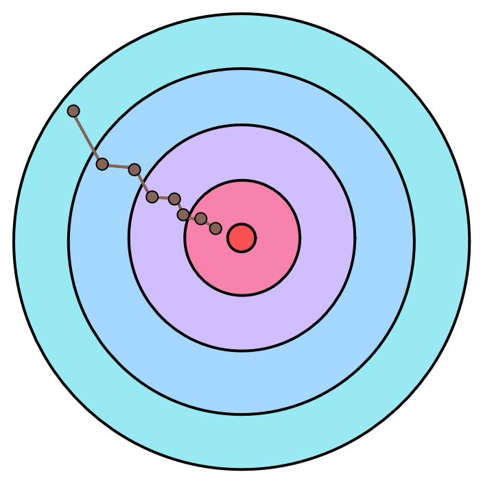
Leibniz again: one does not jump to the minimum; one descends through progressive transformations. The path zigzags towards the bottom, overshooting at each step and correcting itself.

$$ \hat{\theta} = \theta - \eta \cdot \nabla L(\theta)$$

where $\hat{\theta}$ is the newly updated parameter and $\eta$ (learning rate) is the step length.

Make the origami, unmake the origami, redo the origami, unmake the origami….

If we think of the neural network drawn in the first part (we count 26 parameters) it becomes hard to visualise a surface to traverse, even for those accustomed to “thinking four-dimensionally”.

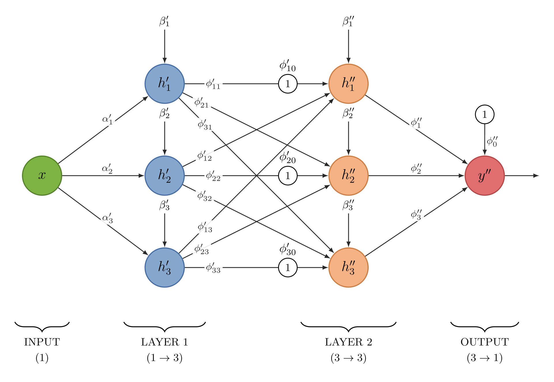
But it is not necessary to do so. We know that after every negative verdict I must unmake the origami and then redo it, until someone tells us: “yes, it looks like a cuddly teddy bear”. We already have everything: the photo of the teddy bear as the reference to reach, the folds as the transformation process, my son as the instrument to measure the distance from that reference, and the unmaking to understand which folds caused the error before starting over.

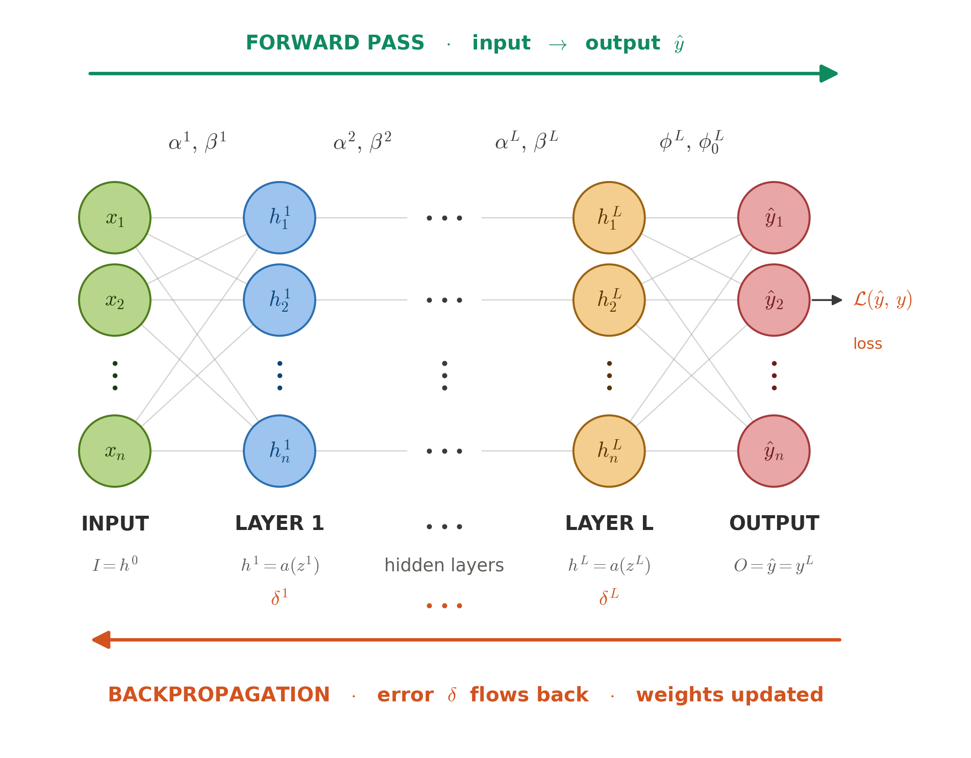
In the case of the network, the photo of the teddy bear is the dataset: a collection of examples in which every input is associated with its expected real value, the ground truth. The folds correspond to forward propagation, the sequence of calculations that traverses the layers from part 1. My son is the loss function, which measures the distance between the model’s prediction and the ground truth. The unmaking to understand where to correct is backpropagation: the algorithm that goes back through the layers in reverse to identify the parameters responsible for the error and calculate by how much to correct them.

Let us try to visualise how the derivatives would be handled in a network with three layers:

• Forward Pass

  $$ \begin{align*} z_0 &= \beta_0 + x \cdot \alpha_0 \\ h_1 &= a(z_0) \\ \\ z_1 &= \beta_1 + h_1 \cdot \alpha_1 \\ h_2 &= a(z_1) \\ \\ z_2 &= \beta_2 + h_2 \cdot \alpha_2 \\ h_3 &= a(z_2) \\ \\ \hat{y} &= \phi_0 + \phi_1 \cdot h_3 \ (\text{output}) \\ \mathcal{L}_i& = (\hat{y} - y_i)^2 \ (\text{loss function}) \end{align*} $$

  so in the end we will have the composition of the loss as a series of composed functions:

  $$ \mathcal{L}_i = \left\{[ \phi_0 + \phi_1 \cdot a(\beta_2 + a(\beta_1 + a(\beta_0 + x \cdot \alpha_0) \cdot \alpha_1) \cdot \alpha_2) ] - y_i \right\}^2 $$

• Backward Pass

  The derivative of $\mathcal{L}_i$ with respect to each intermediate variable follows, in reverse order

  $$ \begin{gathered} \boxed{\longleftarrow} \\[8pt] \frac{\partial \mathcal{L}_i}{\partial z_0} \underset{\frac{\partial h_1}{\partial z_0}}{\longleftarrow} \frac{\partial \mathcal{L}_i}{\partial h_1} \underset{\frac{\partial z_1}{\partial h_1}}{\longleftarrow} \frac{\partial \mathcal{L}_i}{\partial z_1} \underset{\frac{\partial h_2}{\partial z_1}}{\longleftarrow} \frac{\partial \mathcal{L}_i}{\partial h_2} \underset{\frac{\partial z_2}{\partial h_2}}{\longleftarrow} \frac{\partial \mathcal{L}_i}{\partial z_2} \underset{\frac{\partial h_3}{\partial z_2}}{\longleftarrow} \frac{\partial \mathcal{L}_i}{\partial h_3} \underset{\frac{\partial \hat{y}}{\partial h_3}}{\longleftarrow} \frac{\partial \mathcal{L}_i}{\partial \hat{y}} \longleftarrow \mathcal{L}_i \end{gathered} $$

  The connection between all these derivatives follows the chain rule. If $\mathcal{L}$ depends on $h_1$ and $h_1$ depends on $z_0$, the derivative with respect to $z_0$ is obtained by multiplying the derivatives along the path.

  $$\frac{\partial \mathcal{L}}{\partial z_0} = \frac{\partial \mathcal{L}}{\partial h_1} \cdot \frac{\partial h_1}{\partial z_0}$$

  Each arrow in the diagram is one of these local derivatives. Travelling the chain from right to left and multiplying, we trace back to the derivative with respect to the parameters.

And now let us put all the formulas together, generalising a little.

• Input

  • $I$: input vector with $n$ features; in the network it is simply layer 0 of input: $h^{0} = I$
  • $O$: output of the network, i.e. $\hat{y}$
  $$ I = \{x_1, \ldots, x_n\} \qquad O = \hat{y} $$

• Forward Pass

  • step 1

    Pre-activation (layer $l$, unit $k$, for $l = 1, \ldots, L$)

    $$ z_k^{l} = \beta_k^{l} + \sum_{j=1}^{n_{l-1}} \alpha_{kj}^{l} \cdot h_j^{l-1} $$

    with $h_j^{0} = x_j \in I$ at the first layer.

  • step 2

    Activation (layers $l = 1, \ldots, L$)

    $$ h_k^{l} = a\left(z_k^{l}\right) $$

    The vector $h^l = (h_1^l, \ldots, h_{n_l}^l)$ becomes the input of the next layer. Steps 1 and 2 are repeated up to layer $L$.

  • step 3

    Output (only at the final layer)

    $$ \hat{y} = \phi_0 + \sum_{k=1}^{n_L} \phi_k \cdot h_k^{L} $$

    The weights $\phi$ appear only here.

  • step 4

    Loss (for sample $i$)

    $$ \mathcal{L}_i = \left(\hat{y} - y_i\right)^2 $$

• Backward Pass

  • step 1

    Error signal at the output (layer $L$)

    We define $\delta_k^{l} = \frac{\partial \mathcal{L}}{\partial z_k^{l}}$: the derivative of the loss with respect to the pre-activation of unit $k$ at layer $l$, corresponding to the terms $\frac{\partial \mathcal{L}_i}{\partial z_l}$ from the previous example.

    $$ \delta_k^{L} = \frac{\partial \mathcal{L}}{\partial \hat{y}} \cdot \phi_k \cdot a'\left(z_k^{L}\right) $$

  • step 2

    Backward propagation (from $L-1$ down to 1)

    $$ \delta_k^{l} = \left(\sum_{m=1}^{n_{l+1}} \alpha_{mk}^{l+1} \cdot \delta_m^{l+1}\right) \cdot a'\left(z_k^{l}\right) $$

  • step 3

    Parameter gradients

    $$ \begin{align*} \frac{\partial \mathcal{L}}{\partial \alpha_{kj}^{l}} &= \delta_k^{l} \cdot h_j^{l-1} \\[4pt] \frac{\partial \mathcal{L}}{\partial \beta_k^{l}} &= \delta_k^{l} \\[4pt] \frac{\partial \mathcal{L}}{\partial \phi_k} &= \frac{\partial \mathcal{L}}{\partial \hat{y}} \cdot h_k^{L} \\[4pt] \frac{\partial \mathcal{L}}{\partial \phi_0} &= \frac{\partial \mathcal{L}}{\partial \hat{y}} \end{align*} $$

  • step 4

    Weight update

    $$ (\theta - \eta \cdot \nabla_\theta \mathcal{L}) \rightarrow \theta $$

There is a clarification that, having reached the end, I do not want to let slip. The word AI is often associated with the term algorithm, and here too, in my opinion, the vocabulary has created a problem.

Therefore my clarification is this:

• The model is not an algorithm per se, but a parametric mathematical structure, that is, a composition of functions whose behaviour depends on a set of learned parameters.
• The algorithm does not coincide with the model: it is the procedure that allows one to train it (parameter optimisation) and to execute it (forward pass computation).
• Modern deep learning is not reducible to a single element, but is a system composed of model, optimisation algorithm, objective function and data, which together determine the final behaviour.

In short: the model is what results from training on data, the algorithm is the process that optimises it and puts it into execution, and the data are the starting point from which everything is built.

Acceptable and Negligible

In the first part we built the mathematical structure of a neural network: a composition of simple functions, organised in layers, capable of approximating any continuous function. In this second part we have seen how, within an iterative process, to minimise the error that a neural network makes.

We had promised to give shape to two concepts: acceptable and negligible. And I hope it has become clear where the crux of the matter lies: no matter how much we try to minimise the error made by a model, no matter how many effective optimisation methods have been found, it is not possible to reach the bottom, $\delta = 0$.

Let me repeat: if you hear the words “we are able to reach accuracy percentages close to 100%”, run. If you have no way of doing so, you can reply: “But 100% of which percentage?”.

To conclude, a further clarification is necessary: in this long article we have dealt with a “generic form” of neural network, what it truly is and how it works. But in reality there is not just one type of neural network and there is not just one training method.

Neural networks do one and only one thing well: model a function capable of representing the data just as an ideal mathematical function would. It goes without saying that the data represent something unique and carry with them the innumerable boundary conditions that determine them.

The neural network found for our curve is one type; we will see in a future article how, for classification, we will need to add at the end of our mega composition of functions one last function that changes its output. The way of calculating the error will change. The steps we have seen will not change; it will always be a matter of choosing the layers, the activation function, the most appropriate loss function, and so on.

The type of training is not always the same. We saw an approach in which we have in the dataset examples of output against which to measure the error, but there are other types of training in which these data are not available or the model must measure the error based on “evaluations” of its performance (the models developed for self-driving cars, for example).

And so it is that the concepts of acceptable and negligible take on forms far more complex than they might seem.

The three-body problem

Two bodies that attract each other (a star and a planet) have an orbit that we know how to write down and predict. Add a third and everything changes: the system remains perfectly deterministic, the laws are still the same, no random element, and yet there is no longer a general analytical solution that tells us where the bodies will be at an arbitrary time. A minuscule difference in the initial conditions is enough for the trajectories to diverge.

Deterministic, but unpredictable.

It is exactly what Poincaré wrote, in the passage where the idea of deterministic chaos is effectively born:

“It may happen that small differences in the initial conditions produce very great ones in the final phenomena. A small error in the former will produce an enormous error in the latter. Prediction becomes impossible.” Science and Method (1908)

And yet knowing this has not prevented us from sending probes, satellites and missions into space. On the contrary: it is precisely because we know the limit that we have learned to live with it. By integrating numerically, correcting the course on the fly, keeping the error within known margins. Not by eliminating it, but by knowing within which boundaries we can trust our calculations: making it acceptable and negligible.

I often hear the discussion on deep learning closed with the unreliability due to some or other claim of determinism. But a neural network is deterministic (we have seen it: the mathematics is solid, same weights and same input always give the same output), and yet it remains hard to predict. As with the three-body problem, what breaks down is not determinism but predictability. They are two different things.

The problem is not the last decimal of accuracy we are missing; we have the origami pattern, we see the bear taking shape in all its cuddliness right up to the last instruction. But the problem remains of how we then put this formal system to work. Because in models the error does not live only in training: it lives in use as well. The variance with which we give the inputs transfers to the output; as is often said, garbage in, garbage out.

Acceptable and negligible, then, are not just properties of the model. They are properties of the way in which we choose to use it.

---

A Deep Learning Breviary

Types of neural networks

Question	Type	Explanation
“What value will it have?”	Regression	Predicts a continuous number, for example a price or a temperature.
“Which category does it belong to?”	Classification	Assigns a datum to one or more predefined classes.
“What natural groups exist?”	Clustering	Groups similar data without knowing the categories in advance.
“Which data are anomalous?”	Anomaly detection	Identifies behaviours or values outside the norm.
“What will happen in the future?”	Forecasting	Predicts future events or values from historical data.
“What should I suggest to the user?”	Recommendation	Proposes relevant content, products or services.
“What does this image contain?”	Computer Vision	Recognises objects, people or visual features.
“What does this text mean?”	NLP	Understands, analyses or generates natural language.
“How can I create new content?”	Generation	Produces text, images, audio, video or code.
“What is the best action to take?”	Reinforcement Learning	Learns an optimal strategy through rewards and penalties.

Types of training

Question	Type	Explanation
“Do I have examples with the correct answer?”	Supervised learning	The model learns from already labelled data.
“I have no answers; can I find patterns?”	Unsupervised learning	The model autonomously discovers structures and relations.
“I have few answers and lots of raw data?”	Semi-supervised learning	Combines labelled and unlabelled data.
“Can I create training examples on my own?”	Self-supervised learning	Labels are derived automatically from the data.
“Can I learn by trial and error?”	Reinforcement learning	The model improves by receiving rewards or penalties.
“Is there an existing model I can reuse?”	Transfer Learning	Leverages knowledge learned by a previous model.
“Do I want to specialise an already trained model?”	Fine-Tuning	Adapts a general model to a specific task.
“Must I learn continuously from new data?”	Online / Continual Learning	Progressively updates its knowledge over time.

---

Key terms

• Loss function: measures the distance between the model’s predictions and the real values. Minimising it is the goal of training.
• Mean squared error (MSE): the most common loss function, $L = \frac{1}{N} \sum (y_i - \hat{y}_i)^2$.
• Gradient descent: an algorithm that iteratively updates the parameters in the direction opposite to the gradient of the loss.
• Learning rate $\eta$: the update step in gradient descent.
• Chain rule: the differentiation rule for composite functions, the mathematical foundation of backpropagation.
• Backpropagation: an algorithm that computes the gradients by propagating the error signal backward through the layers.
• Forward pass: the computation that produces the network’s output given an input.
• Backward pass: the computation of the gradients from the output back towards the parameters.
• Hyperparameters: parameters of the training process (learning rate, number of epochs, batch size) that are not learned by the network.
• Batch: a subset of the dataset used to compute the gradient in a single step.
• Epoch: a complete pass through the entire dataset during training.