(How to play with balloons and validate neural networks in the process.)
We have just finished training our model. But the work isn’t over yet. Now we have to figure out whether the training went well.
When evaluating both how the training phase unfolded and the final state the model has reached, two fundamental concepts come into play: overfitting and underfitting.
In the first case the model has adapted itself excessively to the training data. In the second, on the contrary, it wasn’t able to “learn” enough. In both cases we find ourselves faced with a model incapable of generalizing.
In other words, we have to ask ourselves how it will behave when faced with data it has never seen before. If its performance worsens noticeably, it means the learning process didn’t reach the right balance.
To describe this situation, people often resort to a comparison with studying at school. If I study purely by rote, I’ll end up knowing the text without really understanding it. I’ll have learned a sequence of information, but I’ll hardly be able to connect it, reason about it, or apply it to a different context. During an oral exam, then, I’ll easily find myself in trouble as soon as I’m asked a question slightly different from the ones I had prepared.
At the opposite extreme there’s a superficial and fragmentary way of studying. In this case I won’t have acquired even the basic knowledge, and my answers will often be incomplete or inadequate.
The analogy is effective because it describes well the two conditions a model can find itself in. And yet there’s an aspect I consider misleading.
Once again a deeply anthropocentric perspective returns. Protagoras held that «man is the measure of all things», and, in many respects, this idea still influences today the way we explain so-called “machine learning”.
Maybe that’s how it is, maybe it’s a genuine form of learning. In the meantime, though, trying out other points of view does no harm, it isn’t a given that everything might somehow coexist.
Playing with balloons is a serious business
In particular I find it very interesting and fun to understand how, in a system, the micro → macro passage conditions the uncertainty and the equilibrium of the system itself.
Take a balloon, for example. Let’s imagine using a pressure gauge to measure the internal pressure, until we see the instrument’s needle come to rest at $1.2$ atmospheres.
Behind that motionless number, there are billions upon billions of air molecules striking the instrument’s membrane, billions of times per second. Each molecule hits with its own force and speed, and there’s no sense in trying to measure every one of them, all the more so since the needle is much slower than a molecule.
So in the end, what we see in the measurement is the result of the combined effect of all the molecules.
Now, let’s do a thought experiment, let’s shrink the balloon down to a very tiny dot. It has to be small enough to hold only a handful of clearly distinguishable molecules. If we tried to take the measurement now (shrinking the pressure gauge accordingly), we would see the instrument’s needle move erratically. The molecules no longer compensate for one another, each one strikes with its own force and its own speed.
Same gas, same pressure, in the system only how many molecules are read at once changes.
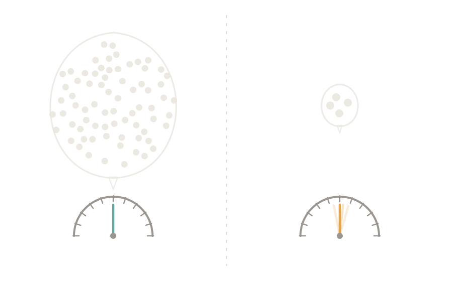
On the left, the large balloon holds many molecules, their impacts compensate for one another and the pressure gauge's needle stays still. On the right, the balloon reduced to very few molecules, each impact carries its own weight and the needle wavers.
It follows, then, that confidence in the measuring system doesn’t come from knowing the molecules one by one, but from how many of them I manage to measure at once.
In a model the measuring instruments are the validation and test phases (the first happens during training, the second once training is complete). If on a classification model I reach a certain accuracy percentage, what does this depend on?
The model is the same, but the stability depends a great deal also on the number of samples.
Some things are much closer to certainty than others
The complete Bertrand Russell quotation is this one: “When one admits that nothing is certain one must, I think, also add that some things are much more nearly certain than others”.
I said I consider the studying example misleading, and I believe this quotation puts us in the right position to look at the point I want to get to. It’s not so important to look at “performance” in itself as at the concept of error, and to do so in the least absolute way possible.
Even though absolute certainty is rare or unattainable, there exist different degrees of reliability of knowledge.
If we want to understand what the error is made of that a model commits on new data, we have to begin by accepting the idea that in practice we will never arrive at the ideal answer.
Let me explain better. We talked about the universal approximation theorem, and more than once we’ve pointed to the terms acceptable and negligible as the most important in the entire world of AI.
And I could start the sentence that follows by writing: “The problem, in fact, is…”, but I really don’t feel like using the word “problem”. I prefer to write that it’s a matter of fact, because we only have data that in themselves represent “dirty” and imperfect answers. But none of this means that we’ll be dealing, in absolute terms, with a precarious system no matter what.
It isn’t the first time I’ve stressed this aspect of AI, but I consider it important, and in every article I’d like to try to convey how wide the neighborhood is that the words negligible and acceptable describe.
In physics this condition is the norm, not the exception. When Millikan measured the charge of the electron, he didn’t “see” it, but observed tiny oil droplets suspended between two charged plates and deduced its value, drop by drop, each one with its own experimental uncertainty.
One estimates the true quantity $\mu$ from imperfect measurements, getting closer and closer to it. Millikan reached it with a small systematic error, corrected by the physicists who came after, up to the extremely high precision of today. Every datum $\mu + \varepsilon$ is the ideal value plus a measurement error $\varepsilon$ that cannot be isolated.
To measure means to infer a quantity that is not directly observable starting from observations affected by error.
Training a model on data is exactly this, that is, chasing a quantity that is never observed in the clear, through measurements that conceal it in the very act of revealing it.
This is the first of three articles. In the first two we’ll try to reflect on the concept of error in a model, and on how the latter, when it becomes too “capable”, becomes like a gas that is too free, ending up “dispersing” itself across too many possible configurations.
In the last article we’ll ask ourselves how a gas is confined and how, in a model, this confinement makes it possible to generalize.
Measuring performance
Before proceeding, I think a clarification is needed on how a model is measured.
The available dataset is divided into three disjoint subsets, each of which performs a specific function in the process of training and evaluating the model.
- Training set: it’s the subset used to optimize the model’s parameters $\phi$. At every iteration of the optimization algorithm, the parameters are updated by minimizing a loss function computed on the examples of the training set. It generally represents the largest portion of the dataset, amounting to roughly 70% or 80% of the available data.
- Validation set: it’s the subset used to estimate the model’s performance during training. At the end of each epoch (one training cycle) the loss, and possibly other metrics, is computed on the validation set without updating the parameters $\phi$. The information obtained is used to guide the training process, for example in selecting the hyperparameters and choosing the best model. Consequently, even though it doesn’t contribute directly to optimizing the parameters, the validation set influences the model indirectly.
- Test set: it’s the subset used exclusively at the end of training to estimate the model’s ability to generalize. Its examples are used neither for optimizing the parameters nor for selecting the hyperparameters. For this reason, the performance measured on the test set constitutes as unbiased an estimate as possible of the performance expected on data not observed during the development of the model.
Few molecules, but good ones
The idea of shrinking a balloon until we can observe the behavior of a few molecules offers an excellent hint.
Let’s follow it, trying to reproduce the same experiment (this time I’d say more artificial than mental) by setting it within a one-dimensional regression. A problem, then, of supervised learning in which we want to estimate a function that describes the relationship between a single independent variable $x$ and a continuous dependent variable $y$.
The goal is to learn a function $f(x)$ starting from a set of pairs of observations $(x_i, y_i)$.
$$ y = f(x) + \varepsilon, $$where $\varepsilon$ represents the error term that accounts for the noise and the components not explained by the model. Once learned, the function can be used to predict the value of $y$ for new values of $x$.
But the aspect of this model that interests us most is the loss we’re going to choose, namely the squared error:
$$ \mathcal{L} = \big( f(x, \phi) - y\big)^2 $$In this way we keep the steps clearly visible.
The square makes the error always positive and allows a particularly simple expansion of the square of the sum: $(a + b)^2 = a^2 + 2ab + b^2$
In practice we’re describing a model similar to the one seen in the first articles (the simplest case is linear regression, in which one assumes that the relationship between the two variables is approximately a straight line).
In this experiment, however, instead of looking for data, we assume that it was obtained from a simple function that generates the answers, to which a random noise is added.
A single dimension. In this way it will be easier to understand how the factors that determine a model’s error interact, in a less dense space.
Nothing new nor original, it’s a method already used in many textbooks. Here, though, I want to place it within a much broader and stranger context than usual.
So, to sum up, the idea is essentially to start from an ideal function we have at our disposal, and then try to measure how far the model departs from it point by point. We can define it as a controlled test bench, from which to try to draw conclusions valid for real cases where we don’t know this ideal function.
Micro and Macro
Let’s fix this image, we’ve already seen it in another article: a gas molecule doesn’t have a fixed position but a range of possible states that the chaotic motion makes uncertain.
In a similar way, the observed value $y$ won’t have a fixed value, but a distribution, and the noise will be the thermal agitation of the datum. The reasons are all very concrete, namely measurement errors, imperfect labels and, more generally, boundary conditions dictated by variables that influence the result but that we have no way of observing.
The key words are these:
- microscopic (the inaccessible): here the equations of classical dynamics are deterministic (for example Newton’s equations for each molecule)
- macroscopic (what is observed): where information about the initial conditions of all the particles is lost and it’s no longer possible to predict a single state, but only a probability distribution
Now, let’s begin by pointing out the three actors at play:
- $f(x, \phi)$ is the model, that is, the prediction produced starting from the input $x$
- $\mathcal{I}(x) = \mu$ is the ideal function, the true quantity we would like to reach
- $y$ is the observed value, the datum we measure
After that let’s try to model this situation mathematically by dividing it into three parts.
First part. The observed value is written as:
$$ y = \mu + \varepsilon $$We’ve already encountered this form along the way in the article, but here we’ll read it in a slightly different manner. In this case the observed value $y$ is given by the sum of the expected ideal value $\mu$ with a random perturbation $\varepsilon$.
Second part. The expected value of the noise is null,
$$ \mathbb{E}(\varepsilon) = 0 $$The symbol $\mathbb{E}$ indicates the expected value, that is, the average of a quantity computed over all its possible values. But why equal to zero and not some arbitrary number?
Let’s start from the definition of noise. The noise is the deviation between the observed value $y$ and the ideal value $\mu$,
$$ \varepsilon = y - \mu $$In turn, the ideal value $\mu$ is by definition the average of the outputs observed for a given input $x$. So we can write
$$ \mathbb{E}(y) = \mu $$Let’s also observe that $\mu$, once an input $x$ is fixed, is a constant. The average of a constant is the constant itself, so
$$ \mathbb{E}(\mu) = \mu $$Putting together what we’ve developed so far we obtain
$$ \mathbb{E}(\varepsilon) = \mathbb{E}(y - \mu) = \mathbb{E}(y) - \mathbb{E}(\mu) = \mu - \mu = 0 $$The intuition behind this expression is actually quite simple. The noise is what’s left after subtracting the average, and what’s left after subtracting the average has zero average.
Let’s take an example to understand well what has just been described. Suppose we weigh several times the same object that we know weighs $1000$ g.
With a good scale we get readings like $998$, $1002$, $999$, $1001$. The values oscillate around $1000$, their average. The deviations with respect to $1000$ are sometimes positive and sometimes negative, and adding them up they tend to compensate for one another. This is zero-mean noise.
Let’s now consider a faulty scale with a tare that always adds $5$ g. The readings become $1003$, $1007$, $1004$ and so on. If we kept considering $1000$ as the ideal value, the deviation would have an average of $+5$ instead of zero. The point is that that $+5$ isn’t random. It’s present in every single measurement and never compensates, so it’s a systematic effect and not an accidental perturbation.
A systematic effect of this kind must be considered signal, not noise. The definition of $\mu$ as the average of the observed outputs accounts for it automatically. With the faulty scale the average of the readings is no longer $1000$ but $1005$, so $\mu = 1005$. With respect to this new value the deviations go back to being distributed around zero, and we recover zero-mean noise.
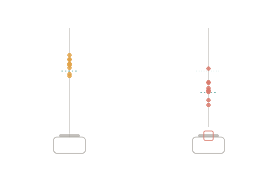
On the left, a correct scale where the readings oscillate symmetrically around the true value (pure noise, zero mean). On the right, a faulty scale with the readings all shifting in the same direction with respect to the true value (bias), while still keeping a spread of their own around the new shifted center.
The moral is the distinction between two different phenomena. The systematic error on the weight corresponds to the bias, that is, a constant error that shifts all the measurements in the same direction. The variation of the readings corresponds to the noise, that is, the unpredictable part that changes from one measurement to another. They are two things that must be rigorously kept separate.
Third part. The variance of the noise is
$$ var(\varepsilon) = \sigma^2 $$$\sigma^2$ represents how large, on average, the space is within which the random variations take place.
Let’s call $\mathbb{E}_y$ the expected value (average) with respect to the noise on the observed value $y$ and rewrite as follows:
$$ \sigma^2 = \mathbb{E}_y \big((\mu - y)^2 \big) $$We can define the variance of the noise as the average of the squared deviations.
At this point we could define the ideal function as the average of the outputs.
With $x$ fixed, the range of possible values of $y$ becomes a probability distribution of $y$ given $x$, that is $Pr(y|x)$.
The ideal function thus becomes the center of mass of this distribution:
$$ \mathcal{I}(x) = \mathbb{E}_y(y) = \int y \cdot Pr(y|x) \, dy $$We could read the formula like this: one takes all the possible values of $y$ (if you’re not familiar with the symbol, the integral sign $\int$ is nothing but a way of summing infinitely many quantities), one weights the probability of each and adds them up. The result will be the value around which the data balance out.
A well-known modern rephrasing of a passage from Aristotle’s Metaphysics says that “the whole is more than the sum of its parts”.
That is, when the elements are combined and interact with one another, there emerge properties, behaviors or characteristics that are not present in the single parts considered in isolation.
What better description for defining the concept $\text{micro} \rightarrow \text{macro}$. We’re not describing the single molecule (the single noisy datum), but a collective property (the average).
The ideal function is a macroscopic quantity that emerges from the microscopic chaos.
Abracadabra
A model, I repeat, is a function $f(x, \phi)$ that, given $x$, produces a prediction.
The parameters $\phi$, however, are not chosen by hand. One arrives at a state in which the parameters take on acceptable values, minimizing the error on the dataset $\mathcal{D}$.
Training looks for the $\phi$ that bring the model’s output closer to the points of $\mathcal{D}$. The relationship of dependence is immediate, the properties of $\phi$ emerge from the model-dataset pair. It’s essentially this aspect that determines the variance.
In the end the goal we want to reach is to demonstrate that it’s possible to “break apart” the expected value of the loss (the average error, taking into account both the noise on the data and the dataset) into the three parts mentioned above:
$$ \text{expected error} = \text{variance} + \text{bias}^2 + \text{noise} $$So let’s make room for the magic.
Let’s start by taking up the loss again:
$$ \mathcal{L}(x) = \big( f(x,\phi) - y \big)^2 $$We don’t see them, but there are two quite distinct errors. One depends on the model and is given by how far the latter departs from the ideal function $\mathcal{I}(x)$. The other error depends on the data and on how “noisy” they are, again with respect to the ideal function.
Let’s add and subtract the ideal function to the loss:
$$ \mathcal{L}(x) = \big( f(x,\phi) - y \big)^2 = \big[ \underbrace{(f(x, \phi) - \mathcal{I}(x))}_{a} + \underbrace{(\mathcal{I}(x) - y)}_b \big]^2 $$We can do this, because if we add and remove the same quantity from an expression, its result doesn’t change.
Let’s look at what we’ve obtained. The term $a$ is the deviation between the model and the ideal function, while the term $b$ is the noise.
Let’s expand the square:
$$ \begin{align} \mathcal{L}(x) &= \big( f(x, \phi) - y \big)^2 \\ &= \big( f(x,\phi) - \mathcal{I}(x) \big)^2 + 2 \big( f(x,\phi) - \mathcal{I}(x) \big) \big( \mathcal{I}(x) - y \big) + \big( \mathcal{I}(x) - y \big)^2 \end{align} $$We’re interested in the average behavior, so let’s apply $\mathbb{E}_y$ (for brevity we use just $f$ for the model and $\mathcal{I}$ for the ideal function):
$$ \mathbb{E}_y [\mathcal{L}(x)] = \underbrace{\mathbb{E}_y [(f - \mathcal{I})^2]}_{t_1} + \underbrace{2\mathbb{E}_y [(f - \mathcal{I})(\mathcal{I} - y)]}_{t_2} + \underbrace{\mathbb{E}_y [(\mathcal{I} - y)^2]}_{t_3} $$Let’s see what happens to each part of the equation.
The first term $t_1$ doesn’t contain $y$ and so must be considered a constant with respect to the noise. The mixed term $t_2$ vanishes, because $\mathbb{E}_y(\mathcal{I} - y)$ equals $\mu - \mu = 0$. The third term $t_3$ is the noise by definition.
What we’ve effectively obtained from the simplification is the following:
$$ \mathbb{E}_y \big[\mathcal{L}(x)\big] = \big( f(x,\phi) - \mathcal{I}(x) \big)^2 + \sigma^2 $$What’s left is represented by the deviation of the model from the ideal and the noise $\sigma^2$, whose nature we can now see. It’s an element that remains irreducible, no part of the model touches it directly.
And here comes the interesting thing. In gases $\sigma^2$ is the thermal agitation of the datum, the background uncertainty that no “cooling of the model” can eliminate. It’s a sort of unbreachable wall.
Looking inside the deviations
The parameters reach a certain state starting from the training dataset $\mathcal{D}$, so the deviation from the ideal contains two causes. The first is a structural defect that even by averaging cannot be entirely eliminated (this will be the bias). The second is a sampling fluctuation, that natural variation of statistical results one observes when different samples are drawn from the same population (the variance).
Let’s call $f_\mu$ the model’s average prediction over all the possible training datasets that can be drawn from the same phenomenon, and $\mathbb{E}_{\mathcal{D}}$ the expected value (average) with respect to the choice of the dataset $\mathcal{D}$.
So let’s write:
$$ f_{\mu}(x) = \mathbb{E}_{\mathcal{D}} \big( f(x,\phi_{\mathcal{D}}) \big) $$Let’s pause for a moment to understand the difference between the two averages, because it’s the heart of the whole reasoning. Let’s imagine fixing a single input $x$. The average over the noise $\mathbb{E}_y$ corresponds to redoing the measurement many times right there where the datum $y$ oscillates because of the noise, while the model and the dataset stay the same. The average over the dataset $\mathbb{E}_{\mathcal{D}}$ is another thing, because this time we keep the point $x$ fixed but each time we reshuffle the training dataset, retrain the model and look at the new prediction. In the first case what varies is the datum, in the second what varies is the model.
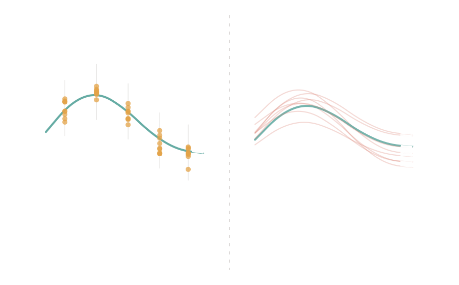
On the left, the model stays fixed (the curve) while the observed datum oscillates because of noise. This is the average over the noise, computed by repeating the measurement with the same model. On the right, the point stays fixed but it's the model that changes with every different dataset. In this case we're talking about the average over the dataset, where the highlighted curve is the typical prediction around which the others are distributed.
Let’s take an example to make everything clearer. Let’s take a hundred different datasets, but ones that describe the same phenomenon. We use these data to train our model. We obtain a hundred curves slightly different from one another. Their average, point by point, is precisely $f_\mu$, the typical prediction, what the model says on average independently of the particular dataset. The variance is the way the curves move around this average.
Here too we use the same trick:
$$ \begin{align} \big( f(x,\phi_{\mathcal{D}}) - \mathcal{I}(x) \big)^2 = \big[ \underbrace{(f(x,\phi_{\mathcal{D}}) - f_{\mu}(x))}_{a} + \underbrace{(f_{\mu}(x) - \mathcal{I}(x))}_b \big]^2 \end{align} $$In this case too we have an expression divided into two parts. The term $a$ is the specific deviation of the model from the typical prediction (the fluctuation), while the term $b$ is the deviation of the typical prediction from the ideal (the structural defect).
Here too we expand (using $f$ for $f(x,\phi_{\mathcal{D}})$):
$$ (f - \mathcal{I})^2 = (f-f_\mu)^2 + 2(f-f_\mu)(f_\mu-\mathcal{I}) + (f_\mu-\mathcal{I})^2 $$Let’s apply the average:
$$ \mathbb{E}_{\mathcal{D}}\big[(f - \mathcal{I})^2\big] = \underbrace{\mathbb{E}_{\mathcal{D}}[(f-f_\mu)^2]}_{t_1} + \underbrace{2\mathbb{E}_{\mathcal{D}}[(f-f_\mu)(f_\mu-\mathcal{I})]}_{t_2} + \underbrace{\mathbb{E}_{\mathcal{D}}[(f_\mu-\mathcal{I})^2]}_{t_3} $$Here too let’s check each term.
The first term $t_1$ is the variance, the dispersion of the predictions around the average, that is, how much the predictions jitter as the dataset changes. It defines the instability given by the excessive dependence on the sample, because changing the dataset changes the result.
The mixed term $t_2$ vanishes in this case too, but for a slightly different reason. Indeed, the factor $(f_\mu-\mathcal{I})$ is independent of the dataset $\mathcal{D}$ and can therefore be taken outside the computation of the average.
$$ (f_\mu-\mathcal{I})\,\mathbb{E}_{\mathcal{D}}(f-f_\mu). $$What remains is precisely:
$$ \mathbb{E}_{\mathcal{D}}(f-f_\mu) = \mathbb{E}_{\mathcal{D}}(f)-f_\mu = f_\mu-f_\mu = 0, $$from which it immediately follows that $t_2=0$.
The third term $t_3$ is the bias squared, it doesn’t depend on the dataset and represents the structural error present even if we used an infinite number of data. It depends, in fact, on the “shape” of the model, not on the scarcity of the data, and represents how far the typical prediction remains from the ideal.
Tying up the threads
Let’s broaden the representation of the average behavior by adding the last expression:
$$ \mathbb{E}_{y,\mathcal{D}}\big[\mathcal{L}(x)\big] = \underbrace{ \mathbb{E}_{\mathcal{D}}\big[ \big( f - f_{\mu} \big)^2 \big]}_{\text{variance}} + \underbrace{\big(f_{\mu}(x) - \mathcal{I}(x)\big)^2}_{\text{bias}^2} + \underbrace{\sigma^2}_{\text{noise}} $$Where the variance indicates the uncertainty due to the sampled dataset, the square of the bias represents the departure from the ideal and finally the noise is given by the intrinsic uncertainty of the data.
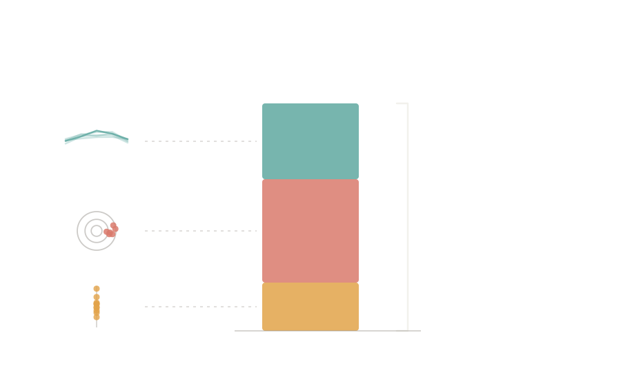
The three contributions that add up in the expected error of a model: the variance (at the top, teal, how much the predictions change as the dataset varies), the bias squared (in the middle, coral, how far the typical prediction remains from the ideal) and the noise (at the bottom, amber, the intrinsic uncertainty of the data, irreducible). Stacked, they give the overall expected error.
We’ve opened a circle and now we necessarily have to close it.
A model with high bias is the one we said was in underfitting, because the typical prediction remains far from the ideal regardless of the data. And this is a defect in the model’s shape, not a question of how much data it has seen.
A model with high variance is instead in overfitting, the gas that’s too free we were talking about, because it clings to the particular dataset and it’s enough to reshuffle the data for the prediction to change. The noise, finally, doesn’t depend on either of the two, because it’s the thermal agitation of the datum, the part of unpredictability that remains no matter what.
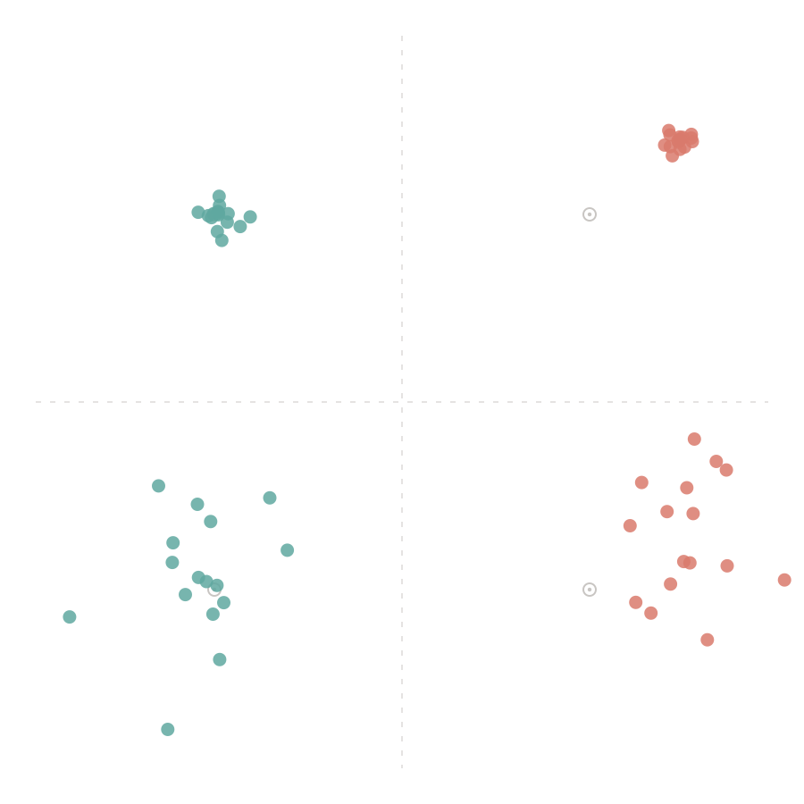
The four ways a model's predictions can arrange themselves with respect to the ideal point (the thin circle in the center). Top left: low bias, low variance, the cloud of points is compact and centered. Top right: high bias, low variance, compact cloud but shifted from the center. Bottom left: low bias, high variance, points scattered but centered on average. Bottom right: high bias, high variance, points scattered and off-center.
Well, in reality we can’t quite close the circle completely yet. We chose a model and a loss simple enough to allow ourselves to follow the reasoning one term at a time. But the additivity of the final expression depends on the loss and therefore doesn’t represent an obvious property a priori.
Let’s be clear, the definitions of underfitting and overfitting remain valid and, for other losses, the three contributions still exist, but they interact in a decidedly more intricate way.
But this will be the subject of the second part of this article.