TypeSafe hasn’t published Jev’s architecture, its weights, or a technical paper. They’ve stated that the model is based on a transformer, that it’s trained only on synthetic data, and that it isn’t autoregressive, meaning it doesn’t produce the answer one token at a time. According to TypeSafe, Jev uses a new architecture with a parallel sampler, produces all the answers in a single query, and evaluates the questions asked on the same state in parallel and independently. The probabilities are calibrated with a post-training step that TypeSafe calls RLCD (Reinforcement Learning for Calibrated Decisions), which compares them with the observed outcomes and corrects them.
It isn’t known whether Jev is an encoder, a decoder, or something else. The hypothesis that it’s built on an LLM (large language model) with public weights circulates among outside observers, but it isn’t confirmed.
What follows is the whole path I took thinking about how to reach the same result.
The final architecture is based on an encoder, but I thought it could be fun to show the whole line of reasoning that led me to rule out the decoder route.
The starting point is a question I asked myself while thinking about Jev: “given that decision problems are very vertical, why not build an architecture on a small BERT-based model, suited to easy and fast fine-tuning?”
Repository
https://github.com/Flab/majev-bb
Important premises
The first, and the most important one. This isn’t a paper, and the architecture described here, a shared encoder, one classification head per question, and temperature scaling to calibrate each of them separately, isn’t a novelty. What I’m covering, then, is a combination of well-known components, from multi-task BERT models like MT-DNN to the intent/slot classifiers used in voice NLU (Natural Language Understanding) systems. What I’m trying to contribute, then, isn’t the architecture itself, but the path taken while playing at reproducing the approach of a system we know nothing about.
The second is that my way of working always starts from the math before moving on to the code. I’ve released the code on github, and I admit it’s the least polished part, so, again, take it all for what it is: an experiment. There’s still the bare minimum needed to try it out, nothing more.
The last premise lies in the fact that I’ve tried to rework all my notes into an organic narrative, an attempt to share reasoning done in the evening on my remarkable, writing scrolls of formulas in a stream-of-consciousness fashion.
If any parts are explained in a not-quite-exhaustive way, questions, remarks, and corrections are welcome.
What emerged from the experiments
I’ll start from the end, from the result of the experiments I ran. It isn’t part of the original set of notes, but it’s interesting because, in a way, it puts into perspective reasoning that was in fact worked out earlier.
The code that comes with the article contains a full experiment. The model reads purchase requests written in Italian and checks whether they comply with the company procedure described in the document itself. There are four questions. The model has to say whether Finance approval is present when the amount requires it, whether there are enough formal quotes, whether the request should be approved, suspended, or rejected, and how urgent it is. The underlying question is whether a model trained only on synthetic documents can hold up on a real one.
The training documents are produced by a script. For each one, evidence is drawn at random (amounts, approvals obtained, quotes, vendor), and the correct answers are obtained by applying the rules of the procedure. The text is generated from templates with several phrasings for each piece of evidence and with sentences deliberately designed to mislead, such as a manager writing “go ahead” in a comment, or a discount offered over the phone and never put in writing. Part of the documents, 250 out of 1,750, are instead written by a local LLM starting from the same evidence.
On the synthetic validation set the model answers correctly between 98 and 100 percent of the time, with well-calibrated probabilities. On the real document it gets two questions out of three right and gets the one about comparing vendors wrong, because it mistakes the discount offered over the phone for a formal quote.
And it gets it wrong confidently, with a probability of 0.85 in the reference run.
To see whether this was an isolated case, I repeated training ten times with different seeds, half with only the template-based documents and half adding the ones written by the LLM. The error shows up in eight cases out of ten, with probabilities between 0.70 and 0.99, while the Finance approval and the final decision always come out correct.
So it isn’t a coincidence, but a limitation of the data. The generator teaches the difference between a formal quote and an informal offer well in the synthetic documents, where the same question gets the right answer almost every time, but not in the form the real document expresses it.
I decided not to fix the dataset precisely because, in this case, I think what went wrong is more instructive, and it points clearly to where the error originates.
And this is exactly where a lesson about calibration comes in too. I’ll keep repeating throughout the rest of the article how important this part is. Temperature scaling is done on the validation set, and if that set is synthetic, the model learns to “trust itself” on synthetic documents. On the real document that confidence means nothing, because the model stays convinced whether it’s right or wrong.
To be able to trust the probabilities on real documents, you have to calibrate on real documents, even if there are only a few.
The repeated runs also brought another aspect to light. On the GPU, training isn’t bit-for-bit reproducible, not even with the same seed, because some operations aren’t deterministic. The scores on the synthetic validation set stay nearly identical, but on the single real document the confidence changes, and sometimes even the answer does. Before drawing conclusions, then, it’s worth training each variant multiple times and looking at the overall trend, keeping in mind that a single real document is a very small test bench.
Rereading the texts produced by the LLM, a problem then came up that I hadn’t anticipated. The prompt gave the urgency level as a score, for example “4/5,” and the LLM copied it straight into the document. For 210 documents out of 250, the answer to the urgency question was therefore written directly in the text, a shortcut no real document offers.
I fixed the prompt so that urgency was described in words instead, and regenerated the data, but the fix in turn had a side effect.
To describe the situation, the prompt used the templates’ own phrasing, and the LLM picked it up almost verbatim, in 24 documents in an almost identical way. The result is that guessing the answer to the urgency question became even easier, with a hundred percent of correct answers on the synthetic data and full confidence on the real one.
Whatever you write in the prompt ends up in the text, and with synthetic data a mistake like this goes unnoticed until you read the examples one by one.
As for costs, training took about two minutes on a laptop GPU and fits in 8 GB of VRAM with a batch size of up to 4. It also works on CPU, where it takes longer (depending on the CPU). Inference on a one-page document, instead, takes about 10 milliseconds on GPU and half a second on CPU.
The repository doesn’t include any pretrained models, and that’s a deliberate choice. Anyone interested can redo the experiment, modify the generator, and see what changes, or start from a minimal generator and a model configuration file to build one for their own domain. The documentation collects the results, the costs, and the log of every change, and suggests a few directions worth exploring.
Problem
Let’s start from a text $x$, which is provided as the shared reference context for all the questions. $Q$ questions are then asked about this same text. Finally, we state that question $q$ admits a finite set of answers, numbered from $1$ to $K_q$.
$$ \mathcal{Y}_q = \{1, \dots, K_q\} $$What we essentially want to obtain, in a Jev-like approach, is a probability distribution over these answers.
That is, a vector described as follows:
$$ p^{(q)}(x) = \big( p^{(q)}_1(x), \dots, p^{(q)}_{K_q}(x) \big), $$- $p^{(q)}_k(x)$: is the probability that the correct answer to question $q$ on text $x$ is the $k$-th one.
- $(q)$: indicates which question the distribution refers to
In addition, every element is greater than or equal to zero, and they sum to 1:
- $p^{(q)}_k(x) \ge 0$
- $\sum_{k=1}^{K_q} p^{(q)}_k(x) = 1$
The system must not generate text. The distribution is used to make decisions, and among other things it will therefore need to be calibrated. In practice, its probabilities will have to match the actual frequencies with which the answers turn out to be correct.
As already mentioned, from here on two different approaches will be followed, one based on the decoder-only architecture, the other on encoder-only.
In general, an encoder-only architecture, like BERT, is designed mainly to understand and represent the meaning of the input. A decoder-only architecture, like GPT, is designed mainly to generate text by predicting one token at a time based on the preceding context.
Both actually originate from the paper that started it all, “Attention Is All You Need,” where they’re described as two parts of a single architecture
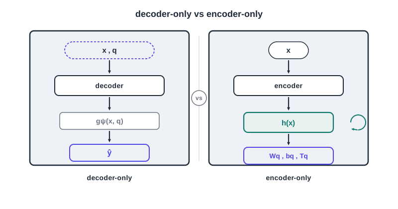
On the left, decoder-only. Text and question enter the sequence together and produce g(x,q), from which the answer ŷ is derived. On the right, encoder-only. The text produces h(x) only once, which is reused for every question by applying the parameters Wq, bq, Tq of the corresponding head.
Both approaches first turn the text into a sequence of tokens, that is, elementary units such as words or parts of words, drawn from a vocabulary $\mathcal{V}$ that contains $|\mathcal{V}|$ tokens.
Decoder approach
In decoder-only approaches, the text and the question, written in natural language, form a single sequence; the decoder then processes it and produces a vector associated with the last position of the sequence, which we define as:
$$ g_\psi(x, q) \in \mathbb{R}^{d'} $$Here $\psi$ denotes the set of the decoder’s parameters and $d'$ the dimension of its internal vectors. The vector depends on both the text $x$ and the question $q$.
Distribution
Starting from the vector produced by the decoder, we can now determine how compatible each possible answer is with the text and the question. To do this, the model uses an output matrix
$$ U \in \mathbb{R}^{|\mathcal{V}| \times d'} $$in which each row corresponds to a token of the vocabulary. The matrix is the same for all questions, but not every token is necessarily a valid answer. For this reason, we only consider the rows associated with the tokens that can represent the answers admitted for question $q$. This part of the matrix is denoted by
$$ U_{\mathcal{Y}_q}. $$The vector produced by the decoder is then combined with the rows of the output matrix associated with the possible answers.
This gives a score for each answer, which is turned into a probability through the softmax function. This way we get a distribution over the possible answers.
$$ p^{(q)}(x) = \mathrm{softmax} \big( U_{\mathcal{Y}_q} \, g_\psi(x, q) \big) $$The softmax turns a vector of real numbers $z = (z_1, \dots, z_K)$ into a probability distribution
$\mathrm{softmax}(z)_k = \frac{\exp(z_k)}{\sum_{k'=1}^{K} \exp(z{k'})}$
where the numerator makes every value positive, and the denominator, the same for every component, makes the sum equal to $1$. The numbers $z_k$ that go into the softmax are called logits.
Causal mask
Encoders and decoders use the same basic mechanism, called self-attention. In this mechanism, each token updates its own representation by taking into account the other tokens in the sequence, giving more weight to the ones it’s most correlated with.
It isn’t always necessary or desirable, though, for a token to be able to look at all the others. To establish which tokens can be considered, a mask is used, represented by a matrix
$$ M \in \mathbb{R}^{L \times L} $$The mask acts on the scores that determine how much each token should consider the others, before these are turned into weights by the softmax.
In particular, the element $M_{ii'}$ indicates whether the token at position $i$ can consider the one at position $i'$. If it’s $0$, token $i'$ can contribute to the representation of token $i$. If it’s $-\infty$, instead, its contribution is excluded, because after the softmax it’s assigned zero weight.
$$ M_{ii'} = \begin{cases} 0 & \text{if } i' \le i \\ \\ -\infty & \text{if } i' > i \end{cases} $$So in a decoder the mask is causal, meaning each token sees only itself and the tokens that precede it.
Reusing the state
Let’s denote by $t_1,\dots,t_L$ the tokens of the sequence and by $H_i$ the representation of the token at position $i$ at the model’s output.
With the causal mask, each token can only use the information that precedes it in the sequence, including itself. In other words, $H_i$ depends only on $t_1,\dots,t_i$ and not on the following tokens.
If the sequence consists of the text followed by the question, the representations of the text’s tokens therefore don’t depend on the question. This means that, once the text has been processed, the information needed to represent it can be computed once and then reused for all subsequent questions.
This is exactly what the KV cache is for. During processing, for every token and every layer, self-attention computes two vectors, called key and value. These vectors are stored in the cache, so they don’t have to be recomputed every time a new question is asked about the same text.
The KV cache can therefore be seen as a kind of shared memory of the text that the decoder can access while processing the various questions. For every token, one key vector and one value vector are stored for each layer. If the text contains $L$ tokens, the cache holds a total of
$2 \cdot n_{\mathrm{layer}} \cdot L \cdot d_{\mathrm{kv}}$
numbers, where the factor $2$ accounts for the key and value vectors, $n_{\mathrm{layer}}$ is the number of layers of the decoder, and $d_{\mathrm{kv}}$ is the dimension of each vector.
As a result, the longer the text, the more memory is needed to store its KV cache.
Restricting the distribution to the admitted answers
Suppose each possible answer $k$ corresponds to a single vocabulary token, which we denote by $\tau_k$.
The decoder assigns a score, called a logit, to each token of the vocabulary. All these values are collected in the vector
$$ u = U\,g_\psi(x,q) \in \mathbb{R}^{|\mathcal{V}|}, $$where $u_{\tau_k}$ is the logit associated with the token $\tau_k$ that represents answer $k$.
Since we’re only interested in the admitted answers, we can ignore the logits of the other tokens and keep only those corresponding to the possible answers. This gives us
$$ p^{(q)}_k(x) = \frac {\exp(u_{\tau_k})} {\sum_{k' \in \mathcal{Y}_q} \exp(u_{\tau_{k'}})} = \frac {P(\tau_k \mid x, q)} {P(\mathcal{Y}_q \mid x, q)} $$Where:
- $P(\tau_k \mid x, q)$: is the probability the decoder assigns to token $\tau_k$ by computing the softmax over the entire vocabulary
- $P(\mathcal{Y}_q \mid x, q) = \sum_{k'} P(\tau_{k'} \mid x, q)$: is the overall probability of all the admitted answers.
The restriction to only the admitted answers can therefore be interpreted as a conditional probability.
In other words, instead of asking what the probability of answer $k$ is among all the tokens of the vocabulary, we ask what its probability is given that the model has produced one of the admitted answers.
The probability the model assigns to tokens that don’t correspond to an admitted answer is therefore excluded. In particular, the quantity
$$ 1-P(\mathcal{Y}_q\mid x,q) $$represents the probability the model had assigned to tokens outside the set of admitted answers.
This probability mass is discarded, and the remaining probabilities are renormalized so that they sum back to 1.
This reasoning is straightforward when each answer corresponds to a single token. When an answer is instead made up of several tokens, we also need to consider how its probability is computed.
Suppose then that answer $k$ is made up of the tokens $\tau_{k,1},\dots,\tau_{k,n_k}$, where $n_k$ denotes the number of tokens in the answer. The probability of the answer is obtained by multiplying the probabilities of the individual tokens, each conditioned on the preceding tokens. In logarithmic form,
$$ \log P(k\mid x,q) = \sum_{r=1}^{n_k} \log P\big( \tau_{k,r}\mid x,q,\tau_{k,1},\dots,\tau_{k,r-1} \big). $$This formulation, however, introduces a problem related to length.
Every probability is at most 1, so its logarithm is less than or equal to 0. Each additional token therefore contributes a non-positive value to the sum. As a result, a longer answer tends to have a lower overall probability simply because it contains more tokens, even when there’s no difference in their meaning.
The probability computed this way therefore introduces a length-related penalty. To compare answers of different lengths, a length-correction rule needs to be introduced.
Cost
To understand how much it costs to process the text and answer the questions, let’s consider the number of operations needed to pass the tokens through the decoder.
Let’s denote by $n_{\mathrm{dec}}$ the number of parameters of the decoder, excluding those of the embeddings, i.e. the vectors associated with the vocabulary tokens. As a first approximation, processing one token through the whole network takes about $2\,n_{\mathrm{dec}}$ operations, because each parameter is used in one multiplication and one addition.
Thanks to the KV cache, the text is processed only once. For each of the $Q$ questions, instead, the decoder only has to process the question’s tokens.
If $L$ is the number of tokens of the text and $L_q$ the number of tokens of question $q$, the overall cost is therefore approximately
$$ C_{\mathrm{dec}} \approx 2\,n_{\mathrm{dec}} \left( L+\sum_{q=1}^{Q}L_q \right) $$The important point is that the length of the text appears only once in the cost, while each question contributes with its own tokens. The KV cache therefore makes it possible to reuse the work already done on the text instead of repeating it for every new question.
Encoder approach
In the encoder-only approach, the text is processed only once, without including the question.
The encoder therefore turns the text into a single vector
$$ h(x)\in\mathbb{R}^{d}, $$with $d=768$, which represents its content in a form the model can use.
Since the question doesn’t enter the encoder, this vector depends only on the text and can be reused for all subsequent questions.
For each question $q$, the model then uses its own linear transformation, learned during training, which takes the vector $h(x)$ and produces a score for each of the $K_q$ possible answers:
$$ p^{(q)}(x) = \mathrm{softmax} \left( \frac{W_q\,h(x)+b_q}{T_q} \right) $$The matrix $W_q\in\mathbb{R}^{K_q\times d}$ contains one row for each answer, while $b_q\in\mathbb{R}^{K_q}$ contains one term associated with each answer.
The product $W_qh(x)$ therefore produces $K_q$ values, one for each possible answer. The temperature $T_q>0$ (we’ll look at exactly what this is later on) controls instead how concentrated or spread out these probabilities turn out to be.
This way, the text is processed only once by the encoder, while for every new question it’s enough to apply the corresponding transformation to the vector already computed.
Having summarized the approach, let’s see how $h(x)$ is obtained and how $W_q$, $b_q$, and $T_q$ are learned and used.
The computation pipeline
$$ x \xrightarrow{\text{tokenizer}} (t_1, \dots, t_L),\, a \xrightarrow{\;E\;} X^{(0)} \xrightarrow{\;f_\theta\;} H \xrightarrow{\text{mean pooling}} h \xrightarrow{\;W_q,\, b_q\;} z^{(q)} \xrightarrow{\;\div T_q,\ \text{softmax}\;} p^{(q)} $$Each arrow represents a computation step, which we can follow starting from the original text:
-
The tokenizer splits the text $x$ into the tokens $t_1,\dots,t_L$ and also produces the attention mask $a$, which indicates which positions contain real tokens and which are instead occupied by filler tokens.
-
The embedding matrix $E$ associates a numerical vector with each token. The resulting vectors are collected in the matrix $X^{(0)}$.
-
The encoder $f_\theta$ processes these vectors taking into account the relations between all the tokens of the sequence and produces the matrix:
$H=f_\theta(X^{(0)},a).$
Each row of $H$ therefore contains the representation of a token after it has been able to take the rest of the sentence into account.
-
Mean pooling summarizes all the representations contained in $H$ into a single vector $h$, which represents the text as a whole.
-
At this point the question $q$ comes into play. The head associated with the question takes $h$ and produces a logit $z^{(q)}$ for each of the possible answers.
-
Finally, the logits are divided by the temperature $T_q$ and passed to the softmax, obtaining the probability distribution $p^{(q)}$ over the answers.
The important point is that all the computation up to $h$ is performed only once, because it depends exclusively on the text.
Only after $h$ does the computation split into $Q$ independent branches, one for each question. In the code, this structure is implemented in the MultiHeadClassifier class in src/model.py.
Tokenizer and embedding
To process several texts together, the sequences need to have the same length, so shorter ones are extended with a special filler token, called padding.
The attention mask is the vector $a = (a_1, \dots, a_L)$ with
$$ a_i = \begin{cases} 1 & \text{if the token at position } i \text{ is part of the text} \\ \\ 0 & \text{if it's a padding token} \end{cases} $$The embedding matrix $E \in \mathbb{R}^{|\mathcal{V}| \times d}$ has a row of $d = 768$ values for every token of the vocabulary. Denoting by $E_{t}$ the row of token $t$, the sequence becomes the matrix:
$$ X^{(0)} = \begin{pmatrix} E_{t_1} \\ \vdots \\ E_{t_L} \end{pmatrix} \in \mathbb{R}^{L \times d} $$in which row $i$ is the embedding of the token at position $i$.
At this point, each row describes an isolated token and contains no information about the rest of the sentence.
Bidirectional encoder
The encoder is mmBERT-base, a multilingual model from the BERT family (Bidirectional Encoder Representations from Transformers).
We denote it by the function $f_\theta$, where $\theta$ is the set of its parameters. It receives $X^{(0)}$ and returns
$$ H = f_\theta(t_1, \dots, t_L) \in \mathbb{R}^{L \times d} $$a matrix with one row $H_i \in \mathbb{R}^{d}$ for each token.
Its self-attention uses a mask that excludes only the padding tokens
$$ M_{ii'} = \begin{cases} 0 & \text{if } a_{i'} = 1 \\ \\ -\infty& \text{if } a_{i'} = 0 \end{cases} $$meaning the token at position $i$ can look at any real token $i'$, whether before or after it. This is why the attention is called bidirectional, and every row $H_i$ depends on the entire text.
mmBERT actually belongs to the ModernBERT family, and this mask holds for 8 of its 22 layers, one every three, which use global attention.
In the other 14, attention is local, so each token only sees the 64 tokens before it and the 64 after it. Since the global layers alternate with the local ones, by the end of the encoder every $H_i$ still depends on the entire text.
Every position contains information about the whole sentence, which is why it makes sense to average them.
Mean pooling
Mean pooling computes the average of the rows of $H$ corresponding only to the real tokens
$$ h = \frac {\sum_{i=1}^{L} a_i \, H_i} {\sum_{i=1}^{L} a_i} \in \mathbb{R}^{d} $$In the numerator, padding tokens have $a_i = 0$ and don’t contribute to the sum, while the denominator counts the real tokens.
The vector $h$ is the system’s shared state and contains $d = 768$ numbers, whatever the length of the text. In a decoder the same operation wouldn’t make sense, because the earlier positions haven’t seen the rest of the text.
The classification heads
For each question $q$ there’s a classification head, that is, a small layer that takes the vector $h$ produced by the encoder and turns it into a score for each of the $K_q$ possible answers.
This transformation is defined by the parameters
$$ W_q\in\mathbb{R}^{K_q\times d} \qquad \text{and} \qquad b_q\in\mathbb{R}^{K_q}. $$During training, a dropout is applied before the classification head. With probability $\rho=0.1$, each component of $h$ is temporarily zeroed out. This pushes the model to spread information across several components of the vector, instead of relying too heavily on a small group of them.
Dropout is a technique used during training to make the model more robust. Before passing to the classification head, some components of the vector $h$ are temporarily and randomly zeroed out. With a dropout of $\rho=0.1$, each component is therefore excluded with a probability of 10%.
The idea is fairly simple. The model can’t always rely on the same components of $h$, but has to learn to spread the information across several components.
This helps reduce the risk of overfitting, that is, the model learning the training data too well and performing worse on new data.
At this point, the classification head turns the vector $h$ into a score for each of the possible answers:
$$ z^{(q)} = W_q \, h + b_q \in \mathbb{R}^{K_q} $$The component $z^{(q)}_k$ is obtained by combining $h$ with row $k$ of $W_q$ and adding the corresponding term of $b_q$.
In particular, the dot product between $h$ and row $k$ of $W_q$ measures how compatible the text’s representation is with that answer. A high value therefore indicates greater compatibility.
The logits are then turned into probabilities through the temperature $T_q$ and the softmax function:
$$ p^{(q)}_k = \frac {\exp\big(z^{(q)}_k/T_q\big)} {\sum_{k'=1}^{K_q}\exp\big(z^{(q)}_{k'}/T_q\big)}. $$The vector $p^{(q)}$ contains exactly $K_q$ probabilities, one for each admitted answer.
No other possible answers are therefore considered, and since each answer corresponds to a single class, there’s no issue with answers made up of several tokens.
The predicted answer is the one to which the model assigns the highest probability:
$$ \hat{y}^{(q)}=\arg\max_k p^{(q)}_k, \qquad \hat{c}^{(q)}=\max_k p^{(q)}_k. $$The quantity $\hat{c}^{(q)}$ represents the confidence, that is, the probability the model assigns to the answer it chose.
It’s worth noting that, once $h$ has been computed, each question is handled separately. The distribution $p^{(q)}$ depends on the text only through $h$, and, for that specific question, only on the parameters $W_q$, $b_q$, and $T_q$. The different questions therefore don’t interact with each other.
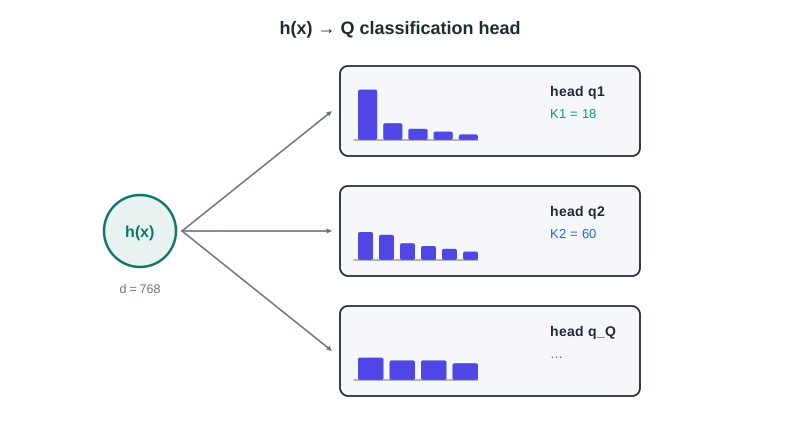
Starting from the same vector h(x), each question has its own independent head: different weights, different softmax, different number of answers. On MASSIVE, the two heads considered have K = 18 and K = 60 possible answers.
One head per type of question
The classification head produces a logit for each possible answer, which is then turned into a probability through the softmax. How these probabilities are interpreted, though, depends on the nature of the answers.
When the answers are distinct, unordered categories, it’s enough to consider the one with the highest probability. If instead there are two possible answers, say no and yes, the softmax produces two probabilities that sum to 1. In this case, the probability of yes can equivalently be expressed as a sigmoid function applied to the difference between the two logits:
$$ p_{\text{yes}} = \frac{1}{1+\exp\big(-(z_{\text{yes}}-z_{\text{no}})\big)} $$When instead the answers represent ordered levels, $v_1 < v_2 < \dots < v_{K_q}$, the probabilities can be interpreted as a distribution along a scale. In this case, besides identifying the most likely level, we can compute the expected value, that is, the average of the levels weighted by their respective probabilities:
$$ \mathbb{E}^{(q)}(x) = \sum_{k=1}^{K_q} p^{(q)}_k(x)\,v_k $$The expected value thus takes the entire distribution into account, not just the level with the highest probability.
For example, if the probability is concentrated on levels 4 and 5, the expected value will lie between these two values, even if neither one necessarily has a probability above 50%.
Parameters
The model’s parameters are collected in
$$ \phi = (\theta, W_1, b_1, \dots, W_Q, b_Q) $$that is, the encoder’s parameters $\theta$ and those of all the heads.
The temperatures $T_1, \dots, T_Q$ are kept separate. The parameters $\theta$ start from the values estimated by mmBERT’s authors during pre-training, the initial training on large amounts of text. The heads start from random values.
The temperatures are estimated last, with $\phi$ fixed.
Why I chose the encoder
The two architectures essentially do the same thing, but in different ways. In the decoder, the question is inserted together with the text and changes the representation the model builds. In the encoder, instead, the text is represented once by a vector $h(x)$, while each question is associated with a small head that turns that vector into probabilities over the possible answers.
The comparison concerns the vertical case, that is, a narrow domain where the questions are known and labeled examples are available.
Computational cost
The encoder reads the text only once. Once $h(x)$ has been obtained, answering a question only means applying the corresponding head, a very small operation.
The decoder, instead, also has to process the question and, above all, is a much bigger model: mmBERT-base has about 110 million parameters excluding embeddings (about 307 million in total, since the 256,000-token vocabulary alone takes up nearly 200 million parameters), while a decoder capable of understanding written questions can have over a billion. The encoder’s advantage therefore grows both with the size of the model and with the number of questions.
A state that gets reused
The encoder compresses the text into a single vector $h$, of 768 values, which can be reused for all the questions.
In the decoder, instead, the text’s representation is kept in a much larger structure, the KV cache. Moreover, with bidirectional attention, adding the question would also change the text’s representation: the cache couldn’t simply be reused, then. In the encoder this problem doesn’t exist, because the question doesn’t enter the sequence: the text is read only once by construction.
Probabilities directly on the answers
In the decoder, probability is initially spread over the tokens of the entire vocabulary and only afterward restricted to the admitted answers. In the encoder, instead, the softmax is applied directly to the possible answers.
This also makes training more direct: the head learns exactly the distribution that will be used at answer time. By minimizing the negative log-likelihood, the model is pushed to assign each answer a probability close to the one observed in the data.
A decoder used without fine-tuning doesn’t have this guarantee: it was trained mainly to predict the next token and to follow instructions, not to produce calibrated probabilities over the domain’s few answers.
One calibration per question
Each question also has its own temperature $T_q$, which makes it possible to calibrate the probabilities separately. In the encoder each head has its own temperature, so this correction doesn’t affect the other questions.
Adapting to the domain
The advantage becomes especially clear when the model has to be adapted to a specific domain. With mmBERT, full fine-tuning is light enough to run on a single graphics card; a decoder with over a billion parameters, instead, needs much more memory and often techniques like LoRA, which make it possible to train only a small part of the parameters.
What gets lost
The encoder is less flexible. It doesn’t understand freely written questions and can’t easily handle a question it has never seen: every new question needs labeled examples and a new head. It also has less general knowledge than a large decoder.
In the vertical case, though, the questions are known and stable. This is why the encoder can turn this very limitation into an advantage, being simpler, cheaper, and more direct.
Notes on training and calibration
Below I’ve reported in full all the notes I took on training and calibration. I had little time to reorganize them, so I hope they’re clear enough.
Training
Loss
The training set contains $N$ examples. Example $j$ consists of a text $x_j$ and a label $y_{j,q} \in \mathcal{Y}_q$ for each question, that is, the correct answer.
Not all examples need to have a label for every question, so it’s a good idea to use an indicator:
$$ \delta_{j,q} = \begin{cases} 1 & \text{if example } j \text{ has the label for question } q, \\ \\ 0 & \text{otherwise}, \end{cases} \qquad N_q = \sum_{j=1}^{N} \delta_{j,q} $$where $N_q$ is the number of examples labeled for question $q$.
The loss for question $q$ is the average NLL (Negative Log-Likelihood Loss) over the labeled examples, and the overall loss is the weighted sum of the individual questions’ losses.
$$ \mathcal{L}_q(\phi) = -\frac{1}{N_q} \sum_{j=1}^{N} \delta_{j,q} \, \log p^{(q)}_{y_{j,q}}(x_j; \phi), \qquad \mathcal{L}(\phi) = \sum_{q=1}^{Q} w_q \, \mathcal{L}_q(\phi) $$In the first formula, $p^{(q)}_{y_{j,q}}(x_j; \phi)$ is the probability the model, with parameters $\phi$, assigns to the correct answer of example $j$.
The logarithm of a probability is negative, so the minus sign makes the loss positive.
The term is $0$ when the model gives probability $1$ to the correct answer, and grows without bound as this probability approaches $0$. In the second formula, $w_q > 0$ is the weight of question $q$, which equals $1$ if not otherwise specified.
If, in a mini-batch, the small group of examples used at each training step, no example is labeled for $q$, the term $\mathcal{L}_q$ is omitted (src/losses.py).
Cooperation between the questions
The heads are isolated, but the encoder is shared. The gradient of the loss with respect to the encoder’s parameters, that is, the vector of derivatives with respect to each parameter in $\theta$, is the weighted sum of the gradients of the individual questions
$$ \nabla_\theta \mathcal{L} = \sum_{q=1}^{Q} w_q \, \nabla_\theta \mathcal{L}_q , $$because the derivative of a sum is the sum of the derivatives. The encoder is therefore changed by all the questions together, and $h$ becomes useful to all of them. The weights $w_q$ control how much each one counts.
Gradient on the logits and overconfidence
For a single example with correct answer $y$ and probability $p = \mathrm{softmax}(z)$, the derivative of the NLL with respect to logit $z_k$ is
$$ \frac{\partial \, (-\log p_y)}{\partial z_k} = p_k - \mathbb{1}[y = k] $$where $\mathbb{1}[y = k]$ equals $1$ if $k$ is the correct answer and $0$ otherwise.
For the correct answer, the derivative equals $p_y - 1$, which is negative, so training raises its logit.
For the other answers it equals $p_k$, which is positive, so training lowers their logits.
I find this part interesting, because the “push” only stops once $p_y = 1$.
On a finite training set, the differences between the logits therefore keep growing, and the model becomes overconfident, that is, more sure of itself than is warranted, on new texts.
This is why calibration is a separate and fundamental step of the architecture.
Optimization
The fine-tuning is full, because it updates all the parameters $\phi$; “supervised,” because it learns from labeled examples. It’s also multi-task, because it trains all the questions on the same encoder.
The following are used:
- AdamW with learning rate $\eta = 3 \cdot 10^{-5}$, the number that controls the size of each update step;
- a warm-up, in which the learning rate grows linearly from $0$ to $\eta$ over the first 10% of the steps, followed by a linear decay down to $0$;
- a weight decay of $\lambda = 0.01$, which slightly shrinks all the parameters at every step to discourage values that are too large;
- a gradient clipping with threshold $\gamma = 1$, which shrinks the gradient when its length exceeds $\gamma$, without changing its direction.
Training proceeds by epochs, that is, complete passes over the training set, for at most 5.
Denoting by $\phi_e$ the parameters at the end of epoch $e$ and by $\mathcal{L}_{q, \mathrm{val}}$ the loss of question $q$ computed on the validation set, early stopping keeps the parameters of the epoch
$$ e^{*} = \arg\min_{e} \sum_{q=1}^{Q} w_q \, \mathcal{L}_{q, \mathrm{val}}(\phi_e) $$that is, the one with the lowest validation loss. Training stops at the first epoch in which the validation loss doesn’t improve, so the minimum is computed over the epochs actually run. The criterion uses the NLL rather than accuracy, the fraction of correct answers, because the goal is the quality of the entire distribution.
Calibration
A head is calibrated when its confidence correctly reflects the probability of being right: among the predictions to which it assigns confidence $c$, about a fraction $c$ should be correct.
To measure this property, the $N_{\mathrm{eval}}$ predictions of the evaluation set are split into $G=10$ groups, called bins, based on confidence.
Bin $B_g$, with $g=1,\dots,G$, collects the predictions with confidence between $(g-1)/10$ and $g/10$.
For each bin, we compare the average confidence, $\mathrm{conf}(B_g)$, and the accuracy, $\mathrm{acc}(B_g)$, that is, the fraction of correct answers.
If, for example, a bin has an average confidence of 0.8, a well-calibrated head should be correct in about 80% of cases.
The ECE (Expected Calibration Error) summarizes these gaps into a single number, giving more weight to bins that contain more predictions:
$$ \mathrm{ECE} = \sum_{g=1}^{G} \frac{|B_g|}{N_{\mathrm{eval}}} \left| \mathrm{acc}(B_g)-\mathrm{conf}(B_g) \right|. $$The lower the ECE, the more consistent the confidence is with the actual frequency of errors.
Temperature scaling
Now, this is the part I consider the most important.
Calibration adds a single parameter to each head, the temperature $T_q > 0$. Before the softmax, all the logits of the head are divided by the same number $T_q$
$$ p^{(q, T_q)}_k(x) = \frac {\exp\big(z^{(q)}_k / T_q\big)} { \sum_{k'=1}^{K_q} \exp\big(z^{(q)}_{k'} / T_q\big) } $$where the superscript $(q, T_q)$ denotes the distribution of question $q$ computed with temperature $T_q$.
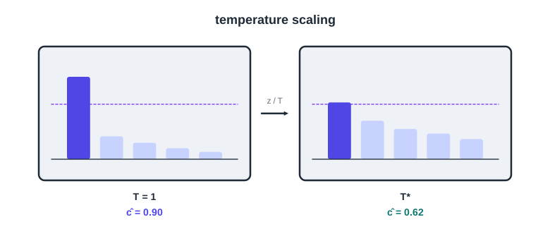
On the left, the raw distribution (T = 1). The confidence ĉ = 0.90 is much higher than the observed frequency (dashed line). On the right, after dividing the logits by the optimal temperature T*, the confidence drops to 0.62 and matches the observed frequency.
The method was proposed by Guo et al. in 2017 (“On Calibration of Modern Neural Networks”)
precisely to correct the excess confidence that modern neural networks can accumulate.
How the temperature is chosen
The temperature is chosen by minimizing the NLL on the validation set. The NLL is well suited to this purpose because it’s a strictly proper scoring rule and therefore rewards probabilities that correctly reflect the data distribution. It’s also a smooth function of the temperature and can be minimized with standard numerical methods.
The ECE doesn’t lend itself as well to optimization. It depends on how the bins are chosen and changes in jumps whenever a prediction moves from one bin to another. The validation set is used instead of the training set because on the training set the network tends to be overly sure of its own predictions.
It’s more convenient to work with the inverse of the temperature,
$$ \beta=\frac{1}{T}. $$For a fixed head, let $z_j=(z_{j,1},\dots,z_{j,K})$ be the logits of example $j$ and $y_j$ the correct answer. The average NLL is
$$ \ell(\beta)= \frac{1}{N_{\mathrm{val}}} \sum_j \delta_j \left( -\beta z_{j,y_j} + \log\sum_k e^{\beta z_{j,k}} \right). $$The parameter $\beta$ controls how much the differences between the logits are reflected in the probabilities. If $\beta$ increases, the distribution becomes more concentrated on the answer with the largest logit. If $\beta$ decreases, the probabilities become more uniform.
The function $\ell(\beta)$ is convex. Its second derivative is in fact an average of the variances of the logits, weighted by the model’s probabilities, and so it can’t be negative. If at least one example has logits that differ from each other, the function is strictly convex and has at most one minimum.
Since $\ell$ is convex, the derivative $\ell'$ is increasing. The minimum exists if $\ell'$ goes from negative to positive values, and to establish this it’s enough to look at what happens at the two extremes of $\beta$.
As $\beta\to0$, that is, $T\to\infty$, the distribution becomes uniform. Every answer has probability $1/K$, and the expected logit coincides with the average of the example’s logits,
$\bar z_j=\frac{1}{K}\sum_k z_{j,k}.$
As a result,
$\ell'(0)= \frac{1}{N_{\mathrm{val}}} \sum_j\delta_j \big(\bar z_j-z_{j,y_j}\big).$
This quantity is negative when, on average, the logit of the correct answer is larger than the average of the logits. This is what we’d expect from a head that has learned to at least partly tell the answers apart.
At the opposite extreme, as $\beta\to\infty$, that is, $T\to0$, the distribution concentrates on the answer with the maximum logit. This gives
$\lim_{\beta\to\infty}\ell'(\beta) = \frac{1}{N_{\mathrm{val}}} \sum_j\delta_j \big( \max_k z_{j,k}-z_{j,y_j} \big) \geq0.$
Each term is zero when the predicted answer is correct and positive when it’s wrong. If the head gets at least one example wrong, the limit is therefore positive.
A finite optimal temperature exists when the head has learned something but also makes some mistakes on the validation set. The other two cases have a simple interpretation. If the head never makes a mistake, the NLL keeps decreasing as $T$ approaches zero, and the optimal temperature would be $T=0$. If instead the logits carry no useful information, the NLL is minimized by letting $T$ go to infinity, making the distribution uniform.
For this reason the search is restricted to the interval
$T_q\in[0.05;\,20].$
The lower bound keeps the temperature from collapsing to zero, while the upper bound keeps it from growing without limit. If the estimated temperature ends up close to either extreme, the result shouldn’t be read as good calibration. It’s rather a sign that the validation set doesn’t contain enough information to estimate a finite temperature.
From output to decisions
For every text and every question the system returns the calibrated distribution:
- the calibrated distribution $p^{(q)}(x)$;
- the predicted answer $\hat{y}^{(q)}$ and its probability $\hat{c}^{(q)}$;
- the expected value $\mathbb{E}^{(q)}(x)$ for
scorequestions.
The probabilities are used to choose the action while taking the cost of errors into account. For a yes/no question, for example, one can choose between acting and not acting. If $\kappa_{\mathrm{FP}}$ is the cost of a false positive and $\kappa_{\mathrm{FN}}$ that of a false negative, it’s worth acting when
$p_{\mathrm{yes}} > \frac{\kappa_{\mathrm{FP}}} {\kappa_{\mathrm{FP}}+\kappa_{\mathrm{FN}}}.$
The threshold therefore depends on the costs of the errors.
This rule is reliable only if the probabilities are calibrated. Calibration is therefore not a detail of the output, but what makes it possible to use it to make decisions.
For the same reason, Jev returns distributions instead of plain labels, and TypeSafe devotes a specific training phase to their calibration, based on a Reinforcement Learning technique it calls RLCD.
Moving to a new domain doesn’t require changing the formulas. All that’s needed is to fix:
- the number of questions $Q$;
- the possible answers $\mathcal{Y}_q$ for each question;
- the type of question and, for
scorequestions, the levels $v_k$; - the weights $w_q$ of the loss.
The dimensions of the matrices $W_q$ and the number of temperatures to calibrate depend on this configuration.
Have fun